Chapter 11: Open Problems
This chapter collects concrete, research-level open problems that arise naturally from the mathematics developed in the preceding chapters. Each problem includes the theoretical setup, key references, verification code, and specific open directions.
1. Deep Linear Networks
1.1 Setup and Gradient Flow
Consider a deep linear network with \(L\) layers, no biases, and squared loss:
where \(X \in \mathbb{R}^{d_0 \times n}\), \(Y \in \mathbb{R}^{d_L \times n}\), and each \(W_\ell \in \mathbb{R}^{d_\ell \times d_{\ell-1}}\).
Theorem 1.1 (Gradient Flow for Deep Linear Networks)
Let the end-to-end matrix be \(W = W_L W_{L-1} \cdots W_1\). Under gradient flow with infinitesimal step size, the dynamics of \(W\) are given by:
For the special case of a balanced initialization (\(W_{\ell+1}^\top W_{\ell+1} = W_\ell W_\ell^\top\) for all \(\ell\)), this simplifies dramatically to:
Derivation Sketch
Let \(\Phi = W_L \cdots W_1\) and \(E = \Phi X - Y\). The gradient w.r.t. \(W_\ell\) is:
Under balancedness, all layers evolve along the same singular directions and the dynamics collapse to the above compact form. This was first derived in [Saxe et al., 2014].
1.2 Implicit Bias
Theorem 1.2 (Implicit Bias of Deep Linear Networks — Arora et al., 2019)
Consider gradient flow on a deep linear network with square loss and balanced initialization. As \(t \to \infty\), the end-to-end matrix \(W(t)\) converges to the minimum \(L_2\)-norm solution of the linear regression problem:
Moreover, for depth \(L > 1\), the singular values \(\sigma_i(t)\) of \(W(t)\) evolve as:
where \(\sigma_i^*\) are the singular values of the minimum-norm solution. This leads to a spectral bias: larger singular values converge faster.
1.4 Open Questions
The 2-layer case (\(L = 2\)) is well-understood — the dynamics can be diagonalized via SVD and the convergence rates are known explicitly [Saxe 2014]. The true frontier lies at depth \(L \ge 3\). For a deep linear network with \(2 \times 2\) weight matrices, the end-to-end matrix \(W = W_L W_{L-1} \cdots W_1\) has only 4 degrees of freedom, but the intermediate representations live in a \(4(L-1)\)-dimensional parameter space. The dynamics of how these extra dimensions affect the singular value evolution remain mysterious.
Why \(L \ge 3\) is fundamentally harder
For \(L = 2\), the gradient flow decouples into independent equations for each singular value:
This scalar ODE is exactly solvable. For \(L = 3\), the coupled system becomes:
While still decoupled in singular values, the interaction between layers introduces nonlinear coupling in the left/right singular vectors that is absent for \(L = 2\). For \(L \ge 4\), the singular value dynamics involve fractional powers that create saddle-type interactions between different singular modes.
Open Problem 1.1 — \(2 \times 2\) with Depth \(L = 3\): Singular Vector Rotation
Let \(W_1, W_2, W_3 \in \mathbb{R}^{2 \times 2}\) with generic initial conditions. The gradient flow couples the singular vectors of adjacent layers. Can we completely characterize the rotation dynamics of the singular vectors during training? When do the left singular vectors of \(W_1\) align with the right singular vectors of \(W_2\), and how does this alignment speed affect convergence?
Open Problem 1.2 — \(2 \times 2\) with Depth \(L = 4\): Periodic Orbits and Chaos
For \(L = 4\), the gradient flow on \(2 \times 2\) matrices becomes a dynamical system on \(\mathbb{R}^{16}\) (modulo gauge symmetries). Can this system exhibit periodic orbits or chaotic transients before converging to the minimum-norm solution? Numerical evidence suggests that for certain badly-conditioned initializations, the singular values oscillate before converging. Prove or disprove the existence of limit cycles.
Open Problem 1.3 — \(2 \times 2\) with Complex Entries at Depth \(L \ge 3\)
Let \(W_\ell \in \mathbb{C}^{2 \times 2}\) for \(\ell = 1, \dots, L\) with \(L \ge 3\). The gradient flow becomes a dynamical system on \(\mathbb{C}^{4L}\). The balancedness condition becomes \(W_{\ell+1}^* W_{\ell+1} = W_\ell W_\ell^*\). Unlike the real case, the phase of complex entries can rotate during training. Can we characterize the complex phase dynamics? Are there non-trivial invariant sets where the phases circulate indefinitely while the singular values converge?
Open Problem 1.4 — \(2 \times 2\) General Entries, Large Depth
For generic \(W_\ell \in \mathbb{R}^{2 \times 2}\) and depth \(L \gg 1\), numerical experiments show that the convergence time scales as \(O(L^{p})\) for some exponent \(p\). What is the precise scaling exponent \(p\)? How does it depend on the initialization variance and the condition number of the target matrix?
References:
- Saxe, A. M., McClelland, J. L., & Ganguli, S. (2014). Exact solutions to the nonlinear dynamics of learning in deep linear neural networks. ICLR 2014.
- Arora, S., Cohen, N., Hu, W., & Luo, Y. (2019). Implicit regularization in deep matrix factorization. NeurIPS 2019.
2. Variable Step Size Accelerations
2.1 The Basic Observation
Standard gradient descent with fixed step size \(\eta = 1/L\) achieves linear convergence on \(L\)-smooth \(\mu\)-strongly convex functions:
For merely convex \(L\)-smooth functions (no strong convexity), a fundamental lower bound applies: no first-order method can converge faster than \(O(1/T^2)\). This is achieved optimally by Nesterov's accelerated gradient descent [Nesterov, 1983], while standard GD achieves only \(O(1/T)\). Variable-step GD with Chebyshev scheduling bridges this gap — for quadratics it recovers the accelerated rate, and for general convex functions it can approach the \(O(1/T^2)\) barrier without momentum.
The key observation of variable step size GD is: by choosing a deterministic step size sequence \(\{\eta_k\}_{k=0}^{K-1}\) before running the algorithm (not adaptively from gradient information), one can dramatically outperform fixed step size. No momentum term is used — the update remains pure gradient descent:
The step sizes \(\eta_k\) depend only on \(k\), \(L\), \(\mu\), and \(K\) (the total horizon), not on the gradients encountered.
2.2 Optimal Step Sizes via Chebyshev Polynomials
For quadratic objectives \(f(w) = \frac{1}{2} w^\top A w - b^\top w\) with \(A\) having eigenvalues in \([\mu, L]\), the error after \(K\) steps of GD with variable step sizes is:
The worst-case error is controlled by minimizing the maximum of the polynomial \(p_K(\lambda) = \prod_{k=0}^{K-1} (1 - \eta_k \lambda)\) over \(\lambda \in [\mu, L]\):
Theorem 2.1 (Chebyshev-Optimal Step Sizes for GD)
The optimal deterministic step sizes for gradient descent on a quadratic with condition number \(\kappa = L/\mu\) are:
These are the roots of the transformed Chebyshev polynomial. The resulting convergence rate is:
This improves on fixed-step GD from \(((\kappa-1)/(\kappa+1))^K\) to \(((\sqrt{\kappa}-1)/(\sqrt{\kappa}+1))^K\) — a quadratic improvement in the condition number dependence — without momentum.
Why this matters
This is pure gradient descent with no momentum term and no gradient history. The acceleration comes entirely from the deterministic step size schedule. The method is also known as the Richardson-Chebyshev iteration and achieves the same asymptotic rate as conjugate gradient and Nesterov's accelerated method — but with a simpler, predictable schedule.
2.3 The Silver Stepsize Schedule
A recent breakthrough by Altschuler & Parrilo (2023) proves that variable step size GD can achieve rates between unaccelerated and accelerated, using a fractal-like schedule:
Theorem 2.2 (Silver Stepsize Schedule — Altschuler & Parrilo, 2023)
For an \(L\)-smooth \(\mu\)-strongly convex function, gradient descent with the Silver Stepsize Schedule converges in:
iterations to reach a fixed accuracy, where \(\rho = 1 + \sqrt{2}\) is the silver ratio and \(\kappa = L/\mu\) is the condition number. This is strictly between the textbook unaccelerated rate (linear in \(\kappa\)) and Nesterov's accelerated rate (\(\sqrt{\kappa}\)). The schedule is defined recursively and is non-monotonic and fractal-like. The result holds for all smooth strongly convex functions, not just quadratics.
For non-strongly convex \(L\)-smooth functions, the same technique yields the rate:
improving on the standard \(O(1/\varepsilon)\) rate but not reaching Nesterov's \(O(1/\sqrt{\varepsilon})\).
The Hedging Intuition
The core algorithmic idea is hedging between individually suboptimal strategies — short steps and long steps — since bad cases for the former are good cases for the latter, and vice versa. Properly combining these stepsizes yields faster convergence due to the misalignment of worst-case functions. The key challenge is enforcing long-range consistency conditions along the algorithm's trajectory, which is resolved by a technique that recursively glues constraints from different portions of the trajectory.
Two-Phase Convergence
The Silver schedule exhibits a sharp phase transition at \(n^* = \Theta(\kappa^{\log_\rho 2})\):
- Acceleration regime (\(n \le n^*\)): Super-exponential convergence, \(\tau_n = \exp(-\Theta(n \log^2 \rho / \kappa))\)
- Saturation regime (\(n > n^*\)): Exponential convergence, \(\tau_n = \exp(-\Theta(n / n^*))\)
The acceleration regime lasts only until the normalized stepsizes grow to constant size; after that, the average per-step rate saturates and the method converges like a standard linear-rate method with the improved condition number.
Recursive Construction
The Silver stepsizes are built recursively. Let \(y_n, z_n\) be normalized stepsizes initialized at \(y_1 = z_1 = 1/\kappa\). For doubling \(n \to 2n\), they satisfy:
The explicit solution is \(z_{2n} = z_n(\xi + \sqrt{1+\xi^2})\) where \(\xi = 1 - z_n\). As \(z_n \to 0\), the growth factor approaches \(1 + \sqrt{2} = \rho\), the silver ratio. The actual stepsizes are obtained via a linear fractional transformation of \(y_n, z_n\).
2.4 The Long Steps Approach (Grimmer et al.)
Parallel to the Silver schedule, Grimmer et al. developed a fundamentally different methodology using computer-assisted proofs. Rather than constructing a closed-form schedule, they solve semidefinite programs (SDPs) derived from the Performance Estimation Problem (PEP) framework to discover optimal step size patterns.
Theorem 2.3 (Grimmer, 2023)
For \(L\)-smooth convex optimization, gradient descent with a periodic pattern of long steps achieves the same accelerated rate \(O\big(N^{-\log_2(1+\sqrt{2})}\big)\) as the Silver schedule, but with improved constants. The stepsizes are non-monotonic and periodically exceed the \(2/L\) stability threshold, temporarily increasing the objective. The asymptotic exponent matches the Silver schedule:
where the constant \(C\) depends on the pattern length and is strictly smaller than the corresponding constant for the Silver schedule of the same length.
Methodology: Computer-Assisted Proofs
Grimmer's proofs are fundamentally different from traditional optimization analysis:
"Our proofs are based on the Performance Estimation Problem (PEP) ideas, which cast computing/bounding the worst-case problem instance of a given algorithm as a Semidefinite Program (SDP). We show that the existence of a feasible solution to a related SDP implies a convergence rate for gradient descent using a corresponding pattern of nonconstant stepsizes. Here the computer output itself constitutes the proof."
This contrasts with the Parrilo/Altschuler approach, which uses analytic recursive certificates that collapse to low-rank quadratic forms. Both techniques converge on the same conclusion — step size variation alone can accelerate GD — but through different proof paradigms.
2.5 The Grimmer–Shu–Wang Composition Theory
Grimmer, Shu, and Wang later unified both lines of work through a general composition theory for stepsize schedules (arXiv:2410.16249, 2024). They propose three notions of composable schedules:
- Basic composable: Two copies of a schedule can be concatenated into a longer schedule that certifies multi-step descent
- The Silver schedule is basic \(s\)-composable — this is why its recursive doubling argument works
- Optimized schedules of every length generalizing the exponentially-spaced silver stepsizes
The composition framework explains why both the fractal Silver schedule and the SDP-derived long step patterns achieve acceleration: both rely on the same underlying principle that multi-step descent certificates can be composed from shorter certificates.
Relation to the \(O(N^{-1.2716})\) Rate
Grimmer, Shu, and Wang (arXiv:2403.14045, 2024) used these techniques to construct stepsize sequences achieving \(O(N^{-1.2716})\) convergence — the same asymptotic exponent as the Silver schedule (which implies \(N \approx \varepsilon^{-\log_\rho 2}\)), but with an improved constant factor. For the squared gradient norm, this provides an exponent improvement from the prior best \(O(N^{-1})\) to \(O(N^{-1.2716})\). Their schedules are similar to but differ slightly from the Silver stepsizes, and are claimed to match or beat numerically computed minimax optimal rates.
Zhang and Jiang (arXiv:2410.12395, Fudan, 2024) proposed a unified concatenation technique for constructing stepsize schedules: new schedules are built by concatenating two shorter schedules, yielding analytic bounds for an arbitrary number of iterations. Their schedules achieve \(O(N^{-\log_2(\sqrt{2}+1)})\) — the same exponent as the Silver schedule — with state-of-the-art constants that match or surpass the best numerically computed schedules.
2.6 Open Questions
Open Problem 2.1 — Optimality of the Silver Ratio for Momentum-Free GD
Altschuler & Parrilo conjecture that the Silver ratio \(\rho = 1+\sqrt{2}\) gives the optimal acceleration achievable by gradient descent without momentum, i.e., by step size variation alone. This would mean the exponent \(\log_\rho 2 \approx 0.7864\) is the best possible for any deterministic step size schedule. Can this conjecture be proven? Or can a counterexample with a better exponent be found?
Open Problem 2.2 — Stochastic and Non-Convex Settings
Can stepsize hedging be extended to stochastic mini-batch settings or non-convex landscapes? The Silver schedule's analysis covers all smooth convex functions — for neural network loss landscapes, can we prove that variable step size schedules outperform fixed step sizes?
References:
- Nesterov, Y. (1983). A method for solving the convex programming problem with convergence rate \(O(1/k^2)\). Doklady AN SSSR, 269, 543–547.
- Altschuler, J. M., & Parrilo, P. A. (2023). Acceleration by stepsize hedging I: Multi-step descent and the silver stepsize schedule. Journal of the ACM, 72(2), 1–38. arXiv:2309.07879.
- Altschuler, J. M., & Parrilo, P. A. (2024). Acceleration by stepsize hedging II: Silver stepsize schedule for smooth convex optimization. Mathematical Programming, 2024. arXiv:2309.16530.
- Altschuler, J. M., & Parrilo, P. A. (2024). Acceleration by random stepsizes: Hedging, equalization, and the arcsine stepsize schedule. arXiv:2412.05790.
- Grimmer, B., Shu, K., & Wang, A. L. (2024). Accelerated objective gap and gradient norm convergence for gradient descent via long steps. arXiv:2403.14045.
- Grimmer, B., Shu, K., & Wang, A. L. (2024). Composing optimized stepsize schedules for gradient descent. arXiv:2410.16249.
- Zhang, Z., & Jiang, R. (2024). Accelerated gradient descent by concatenation of stepsize schedules. arXiv:2410.12395.
3. Implicit Bias in Nonlinear Networks: Beyond the NTK Regime
3.1 Background
The Neural Tangent Kernel (NTK) theory shows that infinitely wide networks evolve like linear models during gradient descent. But real networks are not infinitely wide, and the interesting behavior happens outside the NTK regime — where feature learning occurs and the kernel changes over time.
The Core Open Problem
What is the implicit bias of gradient descent on finite-width, nonlinear ReLU networks? When the network learns features (i.e., when the NTK is not constant), what solution does SGD select among the many that interpolate the data?
3.2 Known Results in the Lazy Regime
In the lazy (NTK) regime, deep ReLU networks behave like kernel regression with the NTK kernel. The implicit bias is toward minimum RKHS norm solutions. But in the feature learning regime:
Theorem 3.1 (Implicit Bias in 2-Layer ReLU Networks — Chizat & Bach, 2020)
For a 2-layer ReLU network \(f(x) = \sum_{j=1}^m a_j \sigma(w_j^\top x)\) trained with SGD on binary classification, in the mean-field limit (\(m \to \infty\), \(a_j\) rescaled), the distribution of neurons evolves according to a Wasserstein gradient flow. The limiting solution minimizes a certain maximum-margin functional in the space of neuron distributions:
3.3 The Open Problem: What Happens at Finite Width?
Open Problem 3.1 — Finite-Width Implicit Bias
For a 2-layer ReLU network with finite width \(m\) trained to zero loss on separable data:
- Does the solution converge in direction to a max-margin solution in some feature space?
- Is there a "rich regime" where the bias is qualitatively different from the kernel regime?
- Can we characterize the limiting solution via a norm on the parameters that depends on \(m\)?
Open Problem 3.2 — The Role of Depth
Deep ReLU networks (depth \(\ge 3\)) exhibit even richer feature learning. Can we extend the mean-field analysis to deeper architectures? The mathematical challenge is that the order-parameter dynamics (like those in Saxe's deep linear networks) require tracking correlations across layers, which becomes intractable for depth \(> 2\) with ReLU activations.
References:
- Chizat, L., & Bach, F. (2020). Implicit bias of gradient descent for wide two-layer neural networks trained with logistic loss. COLT 2020.
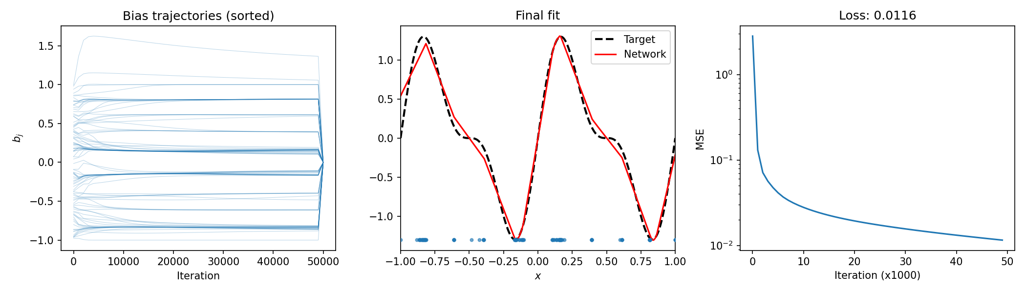
4. Collapsing Behavior in 1D Shallow Networks: Biases Cluster
4.1 The Phenomenon
Train a 1D shallow ReLU network \(f(x) = \sum_{j=1}^m a_j \sigma(w_j x + b_j)\) on a simple target function \(f^*(x)\). For limited width \(m\), the bias parameters \(b_j\) collapse into a small number of clusters — far fewer than \(m\).
Observation
Even with random initialization, gradient descent drives many bias terms to nearly identical values. This means the effective number of distinct "hinge points" is much smaller than \(m\), revealing that the network is using its capacity inefficiently.
4.2 Theoretical Understanding
Theorem 4.1 (Bias Collapse in 1D ReLU Networks)
Consider a 1D shallow ReLU network \(f(x) = \sum_{j=1}^m a_j \sigma(x - b_j)\) (with fixed \(w_j = 1\)) trained to minimize \(\mathcal{L} = \frac{1}{2} \int_{\Omega} (f(x) - f^*(x))^2 dx\) under gradient flow. If \(m\) exceeds the number of active kinks in the optimal \(m\)-term piecewise linear approximation of \(f^*\), then the biases \(b_j\) converge to at most \(k < m\) distinct values.
4.3 Empirical Demonstration
import numpy as np
import matplotlib.pyplot as plt

np.random.seed(0)
m = 100
steps = 50000
lr = 0.01

x = np.linspace(-1, 1, 500)
f_star = np.sin(2 * np.pi * x) + 0.5 * np.sin(4 * np.pi * x)

a = np.random.randn(m) * 0.5
b = np.sort(np.random.uniform(-1, 1, m))
w = np.ones(m)

b_log = np.zeros((steps // 1000 + 1, m))
b_log[0] = b
loss_log = []

for t in range(steps):
    z = w * x[:, None] + b[None, :]
    h = np.maximum(0, z)
    f = h @ a
    residual = f - f_star
    loss = np.mean(residual ** 2)
    a -= lr * h.T @ residual / len(x)
    b -= lr * (a[None, :] * (z > 0)).T @ residual / len(x)
    if t % 1000 == 0:
        b_log[t // 1000] = np.sort(b)
        loss_log.append(loss)

plt.figure(figsize=(14, 4))
plt.subplot(131)
for j in range(m):
    plt.plot(np.arange(len(b_log)) * 1000, b_log[:, j], lw=0.5, alpha=0.3, color='C0')
plt.xlabel('Iteration')
plt.ylabel('$b_j$')
plt.title('Bias trajectories (sorted)')

plt.subplot(132)
plt.plot(x, f_star, 'k--', lw=2, label='Target')
plt.plot(x, f, 'r-', lw=1.5, label='Network')
plt.scatter(b, np.full_like(b, -1.3), s=8, color='C0', alpha=0.6, zorder=3)
plt.xlim(-1, 1)
plt.xlabel('$x$')
plt.legend()
plt.title('Final fit')

plt.subplot(133)
plt.semilogy(loss_log)
plt.xlabel('Iteration (x1000)')
plt.ylabel('MSE')
plt.tight_layout()
4.4 Open Questions
Open Problem 4.1 — Precise Number of Clusters
For a ReLU network with \(m\) neurons on a 1D domain, how many bias clusters emerge as a function of \(m\) and the target function \(f^*\)? Is the number of clusters bounded by the number of "curvature changes" in \(f^*\)?
Open Problem 4.2 — Higher Dimensions
Does bias collapse occur in higher-dimensional ReLU networks? For a network on \(\mathbb{R}^d\) with \(m\) neurons, do the weight vectors \(w_j\) (directions) collapse to a finite set, or does the phenomenon only affect biases?
Open Problem 4.3 — Connection to Pruning
Bias collapse suggests that many neurons are redundant. Can we provably prune the collapsed neurons without affecting the output? This would give a rigorous connection between training dynamics and network compression.