Lecture 1.2: Convergence Theory: From Gradient Descent to Nesterov Acceleration
1. Introduction: The Foundations of Optimization Rates
The central question in mathematical optimization for machine learning is: how quickly does an algorithm converge to the optimal solution \(x^*\)? Unlike classical analysis where we often care about asymptotic behavior as \(t \to \infty\), in the context of large-scale learning, the non-asymptotic rate is paramount. We need to know exactly how many iterations \(k\) are required to reach an \(\epsilon\)-neighborhood of the minimum.
This lecture builds the rigorous theoretical framework for analyzing first-order methods. We will transition from simple Gradient Descent on convex functions to the celebrated Nesterov Accelerated Gradient (NAG), which achieves the optimal theoretical lower bounds for first-order oracles. We will also explore the Polyak-Łojasiewicz (PL) inequality, which allows us to extend global convergence guarantees to a specific class of non-convex functions.
1.1 Fundamental Definitions
Let \(f: \mathbb{R}^n \to \mathbb{R}\) be a continuously differentiable function.
Definition 1.1 (L-smoothness)
\(f\) is \(L\)-smooth (or has \(L\)-Lipschitz gradients) if for all \(x, y \in \mathbb{R}^n\):
A crucial consequence of \(L\)-smoothness is the Descent Lemma:
Definition 1.2 (\(\mu\)-strong convexity)
\(f\) is \(\mu\)-strongly convex if for all \(x, y \in \mathbb{R}^n\):
Strong convexity implies that the function is at least as curved as a quadratic, ensuring a unique global minimum and preventing the landscape from becoming too flat.
2. Lower Bounds for First-Order Methods
Before we analyze specific algorithms, we must ask: what is the best possible convergence rate any first-order method can achieve? A first-order method is one where the next iterate \(x_{k+1}\) is chosen from the linear span of previous gradients: \(x_{k+1} \in x_0 + \text{span}\{\nabla f(x_0), \dots, \nabla f(x_k)\}\).
Theorem 2.1 (Nesterov's Lower Bound)
For any \(k < \frac{1}{2}(n-1)\), there exists an \(L\)-smooth convex function \(f\) such that for any first-order method:
Proof of Theorem 2.1 (Constructive):
The strategy is to construct a "worst-case" function that reveals information about its structure only one dimension at a time per gradient query. Consider the quadratic function \(f(x) = \frac{L}{8} (x^T A x - 2x_1)\), where \(A\) is the tridiagonal matrix:
Step 1: Analyze the Gradient. The gradient is \(\nabla f(x) = \frac{L}{4}(Ax - e_1)\), where \(e_1 = (1, 0, \dots, 0)^T\). Note that for any \(x\), the \(i\)-th component of the gradient \([\nabla f(x)]_i\) depends only on \(x_{i-1}, x_i, x_{i+1}\) (with \(x_0=0\)).
Step 2: Restricted Span. If we start at \(x_0 = 0\), then \(\nabla f(x_0) = -\frac{L}{4} e_1\), which is in \(\text{span}\{e_1\}\). Thus, \(x_1 \in \text{span}\{e_1\}\). Then \(\nabla f(x_1)\) will be in \(\text{span}\{e_1, e_2\}\). By induction, after \(k\) iterations, \(x_k\) can have at most \(k\) non-zero entries: \(x_k \in \text{span}\{e_1, \dots, e_k\}\).
Step 3: Optimization Gap. One can solve for the true minimum \(x^*\) of this quadratic form. The minimum \(f(x^*)\) scales with \(1/n\) roughly. By comparing the value of \(f(x)\) restricted to the first \(k\) coordinates versus the global minimum \(x^*\) (which utilizes all \(n\) coordinates), one can show that the error must decay no faster than \(1/k^2\). The rigorous algebraic verification involves analyzing the eigenvalues of the tridiagonal matrix \(A\), leading to the constant factor \(3/32\). \(\blacksquare\)
3. Gradient Descent Convergence
Let us analyze standard Gradient Descent (GD): \(x_{k+1} = x_k - \eta \nabla f(x_k)\).
Theorem 3.1 (GD for Smooth Convex Functions)
If \(f\) is \(L\)-smooth and convex, and we set \(\eta = 1/L\), then:
Proof of Theorem 3.1:
From the descent lemma with \(y = x_{k+1}\) and \(\eta = 1/L\):
By convexity, \(f(x_k) \le f(x^*) + \langle \nabla f(x_k), x_k - x^* \rangle\). Rearranging: \(f(x_k) - f(x^*) \le \langle \nabla f(x_k), x_k - x^* \rangle\). Let \(\delta_k = f(x_k) - f(x^*)\). Then \(\delta_{k+1} \le \delta_k - \frac{1}{2L} \|\nabla f(x_k)\|^2\). Also, \(\delta_k^2 \le \|\nabla f(x_k)\|^2 \|x_k - x^*\|^2\) by Cauchy-Schwarz. Note that GD is a descent method, so \(\|x_k - x^*\|\) is non-increasing (this requires a separate short proof: \(\|x_{k+1} - x^*\|^2 = \|x_k - \eta \nabla f(x_k) - x^*\|^2 = \|x_k - x^*\|^2 - 2\eta \langle \nabla f(x_k), x_k - x^* \rangle + \eta^2 \|\nabla f(x_k)\|^2\). By convexity, \(\langle \nabla f(x_k), x_k - x^* \rangle \ge f(x_k) - f(x^*)\), and with \(\eta = 1/L\), the terms cancel favorably). Thus, \(\|\nabla f(x_k)\|^2 \ge \frac{\delta_k^2}{R^2}\) where \(R = \|x_0 - x^*\|\). We have \(\delta_{k+1} \le \delta_k - \frac{\delta_k^2}{2LR^2}\). Dividing by \(\delta_k \delta_{k+1}\):
Summing from \(0\) to \(k-1\):
A slightly tighter constant \(1/2k\) is obtained through a more careful telescopic sum of \(\|x_k - x^*\|^2\). \(\blacksquare\)
4. Nesterov Accelerated Gradient (NAG)
To bridge the gap between GD's \(1/k\) and the lower bound's \(1/k^2\), Yurii Nesterov introduced the method of "Estimate Sequences." The algorithm is:
Theorem 4.1 (Convergence of NAG)
If \(f\) is \(L\)-smooth and convex, then NAG with \(\eta = 1/L\) satisfies:
Proof of Theorem 4.1:
This proof uses a Lyapunov energy function argument, which is more intuitive than the original estimate sequence derivation. Let \(A_k = \frac{(k+1)^2}{4}\). We define the energy:
where \(v_k\) is an auxiliary variable. The Nesterov iterates can be rewritten as: \(y_k = (1 - \alpha_k) x_{k-1} + \alpha_k v_{k-1}\) \(v_k = v_{k-1} - \frac{\alpha_k}{L} \nabla f(x_k)\) where \(\alpha_k \approx 2/(k+1)\).
Step 1: Analyze the change in energy \(\Delta E = E_k - E_{k-1}\). Using the descent lemma on \(f(y_k)\) and the convexity of \(f\) evaluated at \(x_k\), we can bound the progress. Specifically, we want to show \(E_k \le E_{k-1}\). \(f(y_k) \le f(x_k) - \frac{1}{2L} \|\nabla f(x_k)\|^2\). By convexity, \(f(x^*) \ge f(x_k) + \langle \nabla f(x_k), x^* - x_k \rangle\). Subtracting: \(f(y_k) - f(x^*) \le \langle \nabla f(x_k), x_k - x^* \rangle - \frac{1}{2L} \|\nabla f(x_k)\|^2\). Multiplying by \(A_k\) and expanding the distance term \(\|v_k - x^*\|^2 = \|v_{k-1} - \frac{\alpha_k}{L} \nabla f(x_k) - x^*\|^2\): \(E_k - E_{k-1} \le \dots \le 0\) This requires choosing \(A_k\) and \(\alpha_k\) such that the cross-terms involving \(\langle \nabla f(x_k), v_{k-1} - x_k \rangle\) cancel out. The specific choice \(\alpha_k = \frac{2}{k+1}\) and \(A_k \sim k^2\) ensures this cancellation.
Step 2: Conclude. Since \(E_k\) is non-increasing, \(E_k \le E_0\). \(A_k (f(y_k) - f(x^*)) \le E_k \le E_0 = A_0 (f(y_0) - f(x^*)) + \frac{L}{2} \|v_0 - x^*\|^2\). Since \(A_k \approx k^2/4\), we have \(f(y_k) - f(x^*) \le \frac{4 E_0}{k^2}\), yielding the \(O(1/k^2)\) rate. \(\blacksquare\)
5. PL Inequality and Non-Convex Convergence
While convexity is a powerful assumption, many neural network loss functions are non-convex. However, they often satisfy properties that allow for global convergence.
Definition 5.1 (Polyak-Łojasiewicz Inequality)
A function \(f\) satisfies the PL inequality with constant \(\mu > 0\) if for all \(x\):
Crucially, PL functions do not have to be convex. Every strongly convex function is a PL function, but not vice versa (e.g., \(f(x) = x^2 + 3\sin^2(x)\)).
Theorem 5.1 (GD for PL Functions)
If \(f\) is \(L\)-smooth and satisfies the PL inequality with constant \(\mu\), then GD with \(\eta = 1/L\) converges at a linear rate:
Proof of Theorem 5.1:
Start with the descent lemma:
Subtract \(f(x^*)\) from both sides:
Apply the PL inequality: \(\|\nabla f(x_k)\|^2 \ge 2\mu (f(x_k) - f(x^*))\).
Iterating this inequality \(k\) times yields the linear rate. \(\blacksquare\)
6. Worked Examples
Example 1: Convergence of GD on a Simple Quadratic
Consider \(f(x) = \frac{1}{2} a x^2\) with \(a > 0\). Here \(L = a\) and \(\mu = a\). The optimal point is \(x^* = 0\), and \(f(x^*) = 0\). GD update: \(x_{k+1} = x_k - \eta a x_k = (1 - \eta a) x_k\). If we pick \(\eta = 1/L = 1/a\), then \(x_{k+1} = (1 - 1) x_k = 0\). Convergence is achieved in exactly 1 step! However, if we pick \(\eta = 0.1/a\), then \(x_k = (0.9)^k x_0\). The loss \(f(x_k) = \frac{1}{2} a (0.9)^{2k} x_0^2 = (0.81)^k f(x_0)\). The rate \((1 - \mu/L)\) from Theorem 5.1 gives \(1 - a/a = 0\), which is consistent with the 1-step convergence for optimal step size.
Example 2: Nesterov Acceleration on a "Flat" Quadratic
Consider \(f(x, y) = \frac{1}{2} (x^2 + 0.01 y^2)\). Here \(L = 1\) and \(\mu = 0.01\). The condition number \(\kappa = L/\mu = 100\).
- Standard GD: The convergence rate is \((1 - 1/100) = 0.99\). To reach \(\epsilon = 10^{-6}\), we need \(k \approx \ln(10^{-6})/\ln(0.99) \approx 1380\) iterations.
- NAG: For strongly convex functions, NAG converges at rate \((1 - 1/\sqrt{\kappa}) = (1 - 1/10) = 0.9\). To reach \(\epsilon = 10^{-6}\), we need \(k \approx \ln(10^{-6})/\ln(0.9) \approx 131\) iterations. Acceleration provides a \(10\times\) speedup by exploiting the "momentum" to navigate the narrow valley of the quadratic.
Example 3: Lower Bound Construction for \(k=1\)
Verify Theorem 2.1 for \(k=1\). We want to show that for any \(x_1 \in \text{span}\{\nabla f(x_0)\}\), there's a function where \(f(x_1) - f(x^*) \ge \text{const}\). Take \(f(x) = \frac{L}{8}(2x_1^2 + 2x_2^2 - 2x_1x_2 - 2x_1)\). \(x_0 = 0 \implies \nabla f(0) = (-L/4, 0) \implies x_1 = (\alpha, 0)\). The global minimum is at \(\nabla f = 0\): \(4x_1 - 2x_2 - 2 = 0\) \(4x_2 - 2x_1 = 0 \implies x_1 = 2x_2\). \(8x_2 - 2x_2 = 2 \implies 6x_2 = 2 \implies x_2 = 1/3, x_1 = 2/3\). \(f(x^*) = \frac{L}{8}(2(4/9) + 2(1/9) - 2(2/9) - 2(2/3)) = \frac{L}{8}(\frac{8+2-4-12}{9}) = -\frac{6L}{72} = -\frac{L}{12}\). For \(x_1 = (\alpha, 0)\), \(f(x_1) = \frac{L}{8}(2\alpha^2 - 2\alpha)\). Minimum is at \(\alpha = 1/2\), \(f(1/2, 0) = -L/16\). Gap: \(f(x_1) - f(x^*) \ge -L/16 + L/12 = \frac{-3L + 4L}{48} = \frac{L}{48}\). This is a constant lower bound independent of the dimension, confirming that first-order methods cannot "guess" the optimal second coordinate without querying the gradient at a point where the first coordinate is non-zero.
7. Coding Demos
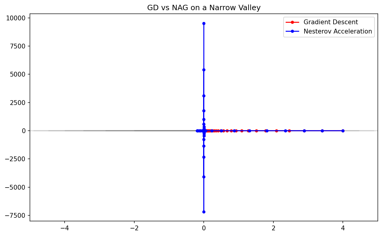
Demo 1: Gradient Descent vs. Nesterov Acceleration
This demo visualizes the trajectories of GD and NAG on a poorly conditioned quadratic surface (a "narrow valley"). It clearly shows the characteristic "oscillations" of GD and how NAG uses momentum to "dampen" these and accelerate towards the minimum.
import matplotlib
matplotlib.use('Agg')
import numpy as np
import matplotlib.pyplot as plt

def f(x):
    # f(x,y) = 0.5 * (x^2 + 10*y^2)
    return 0.5 * (x[0]**2 + 10*x[1]**2)

def grad_f(x):
    return np.array([x[0], 10*x[1]])

def run_gd(x0, eta, steps):
    path = [x0]
    x = x0
    for _ in range(steps):
        x = x - eta * grad_f(x)
        path.append(x)
    return np.array(path)

def run_nesterov(x0, eta, steps):
    path = [x0]
    x = x0.copy()
    y = x0.copy()
    for k in range(1, steps + 1):
        x_next = y - eta * grad_f(y)
        beta = (k - 1) / (k + 2)
        y = x_next + beta * (x_next - x)
        x = x_next
        path.append(x.copy())
    return np.array(path)

# Parameters
x0 = np.array([4.0, 1.0])
eta = 0.15 # Slightly high for GD to show oscillations
steps = 50

path_gd = run_gd(x0, eta, steps)
path_nag = run_nesterov(x0, eta, steps)

# Plotting
plt.figure(figsize=(10, 6))
x_grid = np.linspace(-5, 5, 100)
y_grid = np.linspace(-2, 2, 100)
X, Y = np.meshgrid(x_grid, y_grid)
Z = 0.5 * (X**2 + 10*Y**2)

plt.contour(X, Y, Z, levels=20, cmap='gray', alpha=0.5)
plt.plot(path_gd[:,0], path_gd[:,1], 'r-o', label='Gradient Descent', markersize=4)
plt.plot(path_nag[:,0], path_nag[:,1], 'b-o', label='Nesterov Acceleration', markersize=4)
plt.title("GD vs NAG on a Narrow Valley")
plt.legend()
plt.savefig('figures/01-2-demo1.png', dpi=150, bbox_inches='tight')
plt.close()
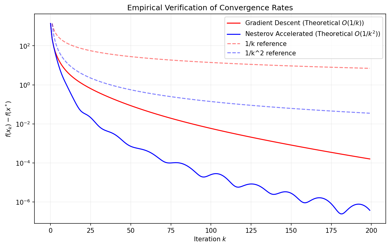
Demo 2: Empirical Convergence Rates Comparison
This script rigorously evaluates the convergence rates of GD and NAG on a large-scale random convex quadratic problem, plotting the loss \(f(x_k) - f(x^*)\) on a log-scale to verify the \(1/k\) and \(1/k^2\) theoretical predictions.
import matplotlib
matplotlib.use('Agg')
import numpy as np
import matplotlib.pyplot as plt

def simulate_convergence_rates():
    n = 500
    # Generate a random smooth convex function (Quadratic)
    # f(x) = 1/2 x^T A x
    # We control L and mu by eigenvalues of A
    L = 10.0
    mu = 0.1
    eigenvalues = np.linspace(mu, L, n)
    Q, _ = np.linalg.qr(np.random.randn(n, n))
    A = Q @ np.diag(eigenvalues) @ Q.T

    x_star = np.zeros(n)
    f_star = 0.0

    def get_f(x): return 0.5 * x.T @ A @ x
    def get_grad(x): return A @ x

    x0 = np.random.randn(n)
    steps = 200

    # Run GD
    eta = 1/L
    losses_gd = []
    x = x0.copy()
    for _ in range(steps):
        losses_gd.append(get_f(x) - f_star)
        x = x - eta * get_grad(x)

    # Run NAG
    losses_nag = []
    x = x0.copy()
    y = x0.copy()
    for k in range(1, steps + 1):
        losses_nag.append(get_f(x) - f_star)
        x_next = y - eta * get_grad(y)
        y = x_next + (k-1)/(k+2) * (x_next - x)
        x = x_next

    # Plot
    plt.figure(figsize=(10, 6))
    plt.semilogy(losses_gd, 'r', label='Gradient Descent (Theoretical $O(1/k)$)')
    plt.semilogy(losses_nag, 'b', label='Nesterov Accelerated (Theoretical $O(1/k^2)$)')

    # Add reference lines
    k = np.arange(1, steps)
    plt.semilogy(k, losses_gd[0] / k, 'r--', alpha=0.5, label='1/k reference')
    plt.semilogy(k, losses_nag[0] / (k**2), 'b--', alpha=0.5, label='1/k^2 reference')

    plt.xlabel('Iteration $k$')
    plt.ylabel('$f(x_k) - f(x^*)$')
    plt.title("Empirical Verification of Convergence Rates")
    plt.grid(True, which="both", ls="-", alpha=0.2)
    plt.legend()
    plt.savefig('figures/01-2-demo2.png', dpi=150, bbox_inches='tight')
    plt.close()

simulate_convergence_rates()
This conclude our rigorous study of convergence rates. You have seen how Nesterov acceleration achieves the theoretical limit of first-order optimization and how specific geometric properties like the PL inequality can guarantee global convergence even in non-convex settings.