9.2 The Representer Theorem and Optimization¶

Introduction¶

In the previous chapter, we established the mathematical foundations of Reproducing Kernel Hilbert Spaces (RKHS). However, the feature space \(\mathcal{H}\) might be infinite-dimensional. How can we perform optimization over an infinite-dimensional space to train machine learning models?

The Representer Theorem bridges this gap. It guarantees that the optimal solution to a large class of regularized empirical risk minimization problems in an RKHS always lies in a finite-dimensional subspace spanned by the kernel evaluated at the training points.

The Generalized Representer Theorem¶

Theorem (Generalized Representer Theorem - Schölkopf, Herbrich, Smola, 2001)

Let \(\mathcal{H}\) be an RKHS over \(\mathcal{X}\) with reproducing kernel \(k\). Given a training set \(\{(x_1, y_1), \dots, (x_n, y_n)\} \subset \mathcal{X} \times \mathcal{Y}\), let \(L: (\mathcal{X} \times \mathcal{Y} \times \mathbb{R})^n \to \mathbb{R} \cup \{\infty\}\) be an arbitrary empirical loss function. Let \(R: [0, \infty) \to \mathbb{R}\) be a strictly monotonically increasing regularization function.

Consider the optimization problem:

\[ \min_{f \in \mathcal{H}} J(f) = L(f(x_1), \dots, f(x_n), y_1, \dots, y_n) + R(\|f\|_\mathcal{H}) \]

Then, any minimizer \(f^* \in \mathcal{H}\) of \(J(f)\) admits a representation of the form:

\[ f^*(x) = \sum_{i=1}^n \alpha_i k(x, x_i) \]

for some coefficients \(\alpha_1, \dots, \alpha_n \in \mathbb{R}\).

Proof:

Step 1: Orthogonal Decomposition. Let \(\mathcal{H}_S = \text{span}\{k(\cdot, x_1), \dots, k(\cdot, x_n)\} \subset \mathcal{H}\) be the subspace spanned by the kernel evaluations at the training data. By the projection theorem in Hilbert spaces, any \(f \in \mathcal{H}\) can be uniquely decomposed as:

\[ f = f_S + f_\perp \]

where \(f_S \in \mathcal{H}_S\) and \(f_\perp \in \mathcal{H}_S^\perp\) (the orthogonal complement). Thus, \(\langle f_\perp, k(\cdot, x_i) \rangle_\mathcal{H} = 0\) for all \(i=1, \dots, n\).

Step 2: Evaluating the Data Points. Applying the reproducing property, the evaluation of \(f\) at any training point \(x_i\) is:

\[ f(x_i) = \langle f, k(\cdot, x_i) \rangle_\mathcal{H} = \langle f_S + f_\perp, k(\cdot, x_i) \rangle_\mathcal{H} \]

By linearity of the inner product:

\[ f(x_i) = \langle f_S, k(\cdot, x_i) \rangle_\mathcal{H} + \langle f_\perp, k(\cdot, x_i) \rangle_\mathcal{H} = f_S(x_i) + 0 = f_S(x_i) \]

Crucially, the empirical loss depends only on the predictions \(f(x_1), \dots, f(x_n)\). Since \(f(x_i) = f_S(x_i)\), the loss term \(L\) is entirely independent of the orthogonal component \(f_\perp\):

\[ L(f(x_1), \dots, f(x_n), Y) = L(f_S(x_1), \dots, f_S(x_n), Y) \]

Step 3: Analyzing the Regularizer. Now consider the RKHS norm of \(f\). Because \(f_S\) and \(f_\perp\) are orthogonal, the Pythagorean theorem in Hilbert spaces dictates:

\[ \|f\|_\mathcal{H}^2 = \|f_S + f_\perp\|_\mathcal{H}^2 = \|f_S\|_\mathcal{H}^2 + \|f_\perp\|_\mathcal{H}^2 \geq \|f_S\|_\mathcal{H}^2 \]

Since \(R(\cdot)\) is strictly monotonically increasing and \(\|f\|_\mathcal{H} \geq \|f_S\|_\mathcal{H}\), it follows that:

\[ R(\|f\|_\mathcal{H}) \geq R(\|f_S\|_\mathcal{H}) \]

Equality holds if and only if \(\|f_\perp\|_\mathcal{H}^2 = 0\), which implies \(f_\perp = 0\).

Step 4: Conclusion. For any \(f = f_S + f_\perp \in \mathcal{H}\), the projected function \(f_S\) achieves the exact same empirical loss but a strictly smaller (or equal) regularization penalty. Therefore, to minimize \(J(f)\) we must have \(f_\perp = 0\), and the optimal solution \(f^*\) lies entirely in \(\mathcal{H}_S\):

\[ f^* = f_S \implies f^*(x) = \sum_{i=1}^n \alpha_i k(x, x_i) \]

\(\blacksquare\)

Implications¶

Instead of optimizing over an infinite-dimensional function space, we only need to optimize over \(n\) scalar coefficients \(\alpha = (\alpha_1, \dots, \alpha_n)^T \in \mathbb{R}^n\). This reduces a problem of calculus of variations to standard vector optimization.

Optimization in SVMs and Duality¶

Support Vector Machines (SVM) are the canonical example of kernel methods.

Primal Formulation¶

The primal optimization problem for a soft-margin SVM in RKHS \(\mathcal{H}\) is:

\[ \min_{f \in \mathcal{H}, b \in \mathbb{R}, \xi \in \mathbb{R}^n} \frac{1}{2} \|f\|_\mathcal{H}^2 + C \sum_{i=1}^n \xi_i \]

Subject to the constraints:

\[ y_i (f(x_i) + b) \geq 1 - \xi_i, \quad \xi_i \geq 0 \quad \forall i \]

Applying the Representer Theorem, we know \(f(x) = \sum_{j=1}^n \alpha_j k(x, x_j)\). The norm is:

\[ \|f\|_\mathcal{H}^2 = \langle \sum_{i} \alpha_i k(\cdot, x_i), \sum_{j} \alpha_j k(\cdot, x_j) \rangle_\mathcal{H} = \sum_{i,j} \alpha_i \alpha_j k(x_i, x_j) = \alpha^T K \alpha \]

where \(K\) is the kernel matrix. The constraint becomes \(y_i (K_i^T \alpha + b) \geq 1 - \xi_i\).

Dual Derivation and Proof¶

To derive the dual, we introduce Lagrange multipliers \(\lambda_i \geq 0\) for the margin constraints and \(\mu_i \geq 0\) for the non-negativity of slacks \(\xi_i\).

Lagrangian:

\[ \mathcal{L}(f, b, \xi, \lambda, \mu) = \frac{1}{2} \|f\|_\mathcal{H}^2 + C \sum_{i=1}^n \xi_i - \sum_{i=1}^n \lambda_i \left[ y_i (f(x_i) + b) - 1 + \xi_i \right] - \sum_{i=1}^n \mu_i \xi_i \]

We can use the reproducing property \(f(x_i) = \langle f, k(\cdot, x_i) \rangle_\mathcal{H}\):

\[ \mathcal{L} = \frac{1}{2} \langle f, f \rangle_\mathcal{H} - \langle f, \sum_{i=1}^n \lambda_i y_i k(\cdot, x_i) \rangle_\mathcal{H} - b \sum_{i=1}^n \lambda_i y_i + \sum_{i=1}^n \xi_i (C - \lambda_i - \mu_i) + \sum_{i=1}^n \lambda_i \]

To find the dual, we minimize \(\mathcal{L}\) with respect to the primal variables \(f, b, \xi\):

Derivative w.r.t. \(f\): Taking the Fréchet derivative with respect to \(f\) in the Hilbert space and setting it to zero:

\[ \nabla_f \mathcal{L} = f - \sum_{i=1}^n \lambda_i y_i k(\cdot, x_i) = 0 \implies f = \sum_{i=1}^n \lambda_i y_i k(\cdot, x_i) \]

Notice this perfectly mirrors the Representer Theorem with \(\alpha_i = \lambda_i y_i\).

Derivative w.r.t. \(b\):

\[ \frac{\partial \mathcal{L}}{\partial b} = - \sum_{i=1}^n \lambda_i y_i = 0 \]

Derivative w.r.t. \(\xi_i\):

\[ \frac{\partial \mathcal{L}}{\partial \xi_i} = C - \lambda_i - \mu_i = 0 \]

Since \(\mu_i \geq 0\), this implies \(0 \leq \lambda_i \leq C\).

Substituting these optimal conditions back into the Lagrangian:

The first two terms become:

\[ \frac{1}{2} \langle \sum_i \lambda_i y_i k(\cdot, x_i), \sum_j \lambda_j y_j k(\cdot, x_j) \rangle_\mathcal{H} - \langle \sum_j \lambda_j y_j k(\cdot, x_j), \sum_i \lambda_i y_i k(\cdot, x_i) \rangle_\mathcal{H} \]

\[ = - \frac{1}{2} \sum_{i,j} \lambda_i \lambda_j y_i y_j k(x_i, x_j) \]

The terms involving \(b\) and \(\xi\) vanish due to the zero-gradient constraints. We are left with the dual objective:

Dual SVM Problem:

\[ \max_{\lambda \in \mathbb{R}^n} \sum_{i=1}^n \lambda_i - \frac{1}{2} \sum_{i=1}^n \sum_{j=1}^n \lambda_i \lambda_j y_i y_j k(x_i, x_j) \]

Subject to:

\(0 \leq \lambda_i \leq C\) for all \(i\)
\(\sum_{i=1}^n \lambda_i y_i = 0\)

This is a concave quadratic programming (QP) problem, which scales with \(n\) but is independent of the dimensionality of \(\mathcal{H}\).

\(\blacksquare\)

Worked Examples¶

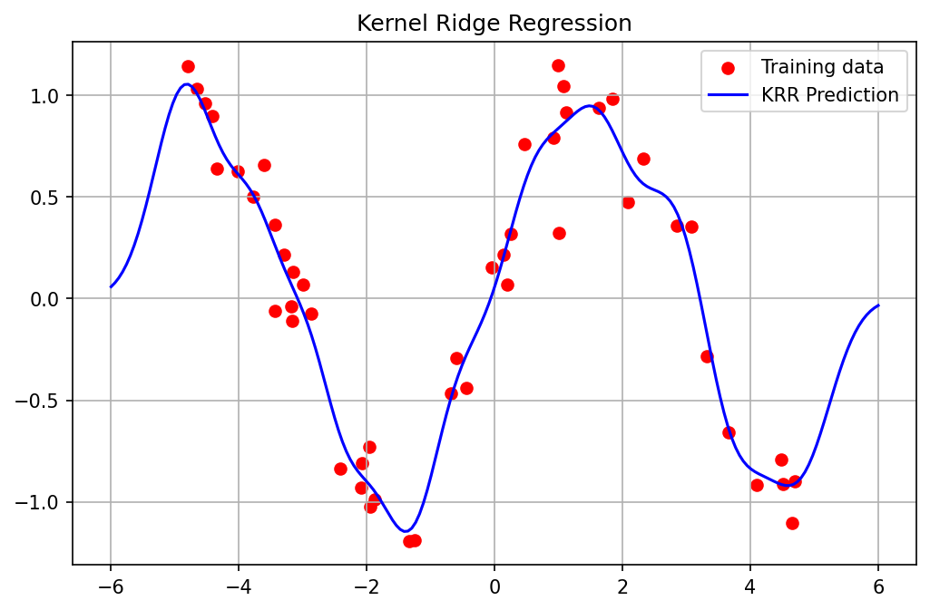
Example 1: Kernel Ridge Regression (KRR)¶

Consider regression with squared loss: \(L(y, \hat{y}) = (y - \hat{y})^2\) and \(L_2\) regularization \(R(\|f\|) = \frac{\lambda}{2} \|f\|_\mathcal{H}^2\). Objective:

\[ J(\alpha) = \|y - K\alpha\|_2^2 + \lambda \alpha^T K \alpha \]

Expanding:

\[ J(\alpha) = y^T y - 2y^T K \alpha + \alpha^T K^2 \alpha + \lambda \alpha^T K \alpha \]

Taking gradient w.r.t \(\alpha\) and setting to 0:

\[ \nabla_\alpha J = -2 K y + 2 K^2 \alpha + 2 \lambda K \alpha = 0 \]

Assuming \(K\) is positive definite, we can multiply by \(K^{-1}\) from the left (or factor out \(2K\)):

\[ (K + \lambda I) \alpha = y \implies \alpha = (K + \lambda I)^{-1} y \]

This provides a closed-form solution for Kernel Ridge Regression!

Example 2: SVM Margin and Support Vectors¶

In the SVM Dual, because of the KKT complementary slackness conditions:

\[ \lambda_i [y_i (f(x_i) + b) - 1 + \xi_i] = 0 \]

If \(0 < \lambda_i < C\), then \(\xi_i = 0\), and \(y_i (f(x_i) + b) = 1\). These points lie exactly on the margin boundary and are called unbound support vectors. We can use any of them to solve for the bias term \(b\):

\[ b = y_i - \sum_{j=1}^n \lambda_j y_j k(x_j, x_i) \]

Points where \(\lambda_i = C\) violate the margin (or are misclassified), called bound support vectors. Points where \(\lambda_i = 0\) do not contribute to the sum \(f(x)\)—they are correctly classified and lie outside the margin.

Example 3: Logistic Regression in RKHS¶

Loss: \(\log(1 + \exp(-y_i f(x_i)))\). By Representer Theorem: \(f(x) = \sum \alpha_i k(x, x_i)\). Optimization: \(\min_\alpha \sum_{i=1}^n \log(1 + \exp(-y_i K_i^T \alpha)) + \frac{\lambda}{2} \alpha^T K \alpha\). This is convex and differentiable, solvable via Newton-Raphson or L-BFGS, entirely avoiding the infinite-dimensional \(\mathcal{H}\).

Coding Demos¶

Demo 1: Kernel Ridge Regression from Scratch¶

Python

import matplotlib
matplotlib.use('Agg')
import numpy as np
import matplotlib.pyplot as plt

def rbf_kernel(X, Y, gamma=1.0):
    X_norm = np.sum(X**2, axis=-1).reshape(-1, 1)
    Y_norm = np.sum(Y**2, axis=-1).reshape(1, -1)
    dists = np.maximum(X_norm + Y_norm - 2 * np.dot(X, Y.T), 0)
    return np.exp(-gamma * dists)

# Generate non-linear data
np.random.seed(42)
X_train = np.sort(np.random.uniform(-5, 5, 50)).reshape(-1, 1)
y_train = np.sin(X_train).ravel() + np.random.normal(0, 0.2, 50)

# KRR Hyperparameters
gamma = 2.0
lambda_reg = 0.1

# 1. Compute Kernel Matrix
K = rbf_kernel(X_train, X_train, gamma)

# 2. Solve for alphas (Representer Theorem)
n = K.shape[0]
alphas = np.linalg.solve(K + lambda_reg * np.eye(n), y_train)

# 3. Predict on test grid
X_test = np.linspace(-6, 6, 200).reshape(-1, 1)
K_test = rbf_kernel(X_test, X_train, gamma)
y_pred = K_test.dot(alphas)

# Plot
plt.figure(figsize=(8, 5))
plt.scatter(X_train, y_train, c='r', label='Training data')
plt.plot(X_test, y_pred, 'b-', label='KRR Prediction')
plt.title("Kernel Ridge Regression")
plt.legend()
plt.grid(True)
plt.savefig('figures/09-2-demo1.png', dpi=150, bbox_inches='tight')
plt.close()

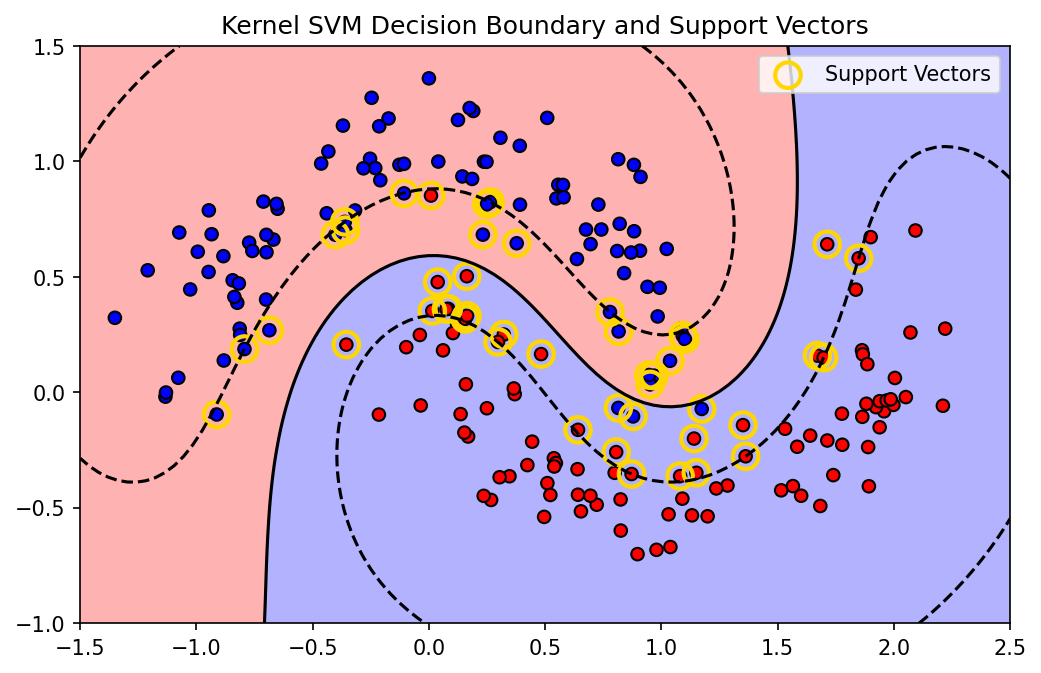
Demo 2: The Sparsity of SVM Support Vectors¶

We demonstrate how the hinge loss induces sparsity in the \(\alpha\) coefficients (the support vectors), unlike KRR which uses all points. We'll use sklearn's SVC which wraps LIBSVM.

Python

import matplotlib
matplotlib.use('Agg')
import numpy as np
import matplotlib.pyplot as plt
from sklearn.svm import SVC
from sklearn.datasets import make_moons

# Create a non-linear classification dataset
X, y = make_moons(n_samples=200, noise=0.15, random_state=42)

# Train Kernel SVM (RBF)
svm = SVC(kernel='rbf', C=1.0, gamma=1.0)
svm.fit(X, y)

# Get support vectors
sv = svm.support_vectors_
dual_coefs = svm.dual_coef_

print(f"Total training points: {X.shape[0]}")
print(f"Number of Support Vectors: {sv.shape[0]}")
print(f"Sparsity: {(1 - sv.shape[0]/X.shape[0])*100:.2f}% of coefficients are strictly zero.")

# Plot decision boundary and highlight support vectors
xx, yy = np.meshgrid(np.linspace(-1.5, 2.5, 100), np.linspace(-1, 1.5, 100))
Z = svm.decision_function(np.c_[xx.ravel(), yy.ravel()])
Z = Z.reshape(xx.shape)

plt.figure(figsize=(8, 5))
plt.contourf(xx, yy, Z, levels=[-10, 0, 10], alpha=0.3, colors=['red', 'blue'])
plt.contour(xx, yy, Z, levels=[-1, 0, 1], linestyles=['--', '-', '--'], colors='k')
plt.scatter(X[:, 0], X[:, 1], c=y, cmap='bwr', edgecolors='k')
plt.scatter(sv[:, 0], sv[:, 1], s=150, facecolors='none', edgecolors='gold', linewidths=2, label='Support Vectors')
plt.title("Kernel SVM Decision Boundary and Support Vectors")
plt.legend()
plt.savefig('figures/09-2-demo2.png', dpi=150, bbox_inches='tight')
plt.close()

Text Only

Total training points: 200
Number of Support Vectors: 46
Sparsity: 77.00% of coefficients are strictly zero.