Chapter 2.4: Kolmogorov-Arnold Networks and Symbolic Approximation Theory¶

1. Introduction: Beyond the MLP Paradigm¶

For decades, the Multilayer Perceptron (MLP) has been the dominant architecture in deep learning. MLPs rely on the Universal Approximation Theorem, using fixed non-linear activations (like ReLU) on nodes and learnable weights on edges. However, in 1957, a profound mathematical theorem was proven that suggests a completely different way to build neural networks.

The Kolmogorov-Arnold Representation Theorem states that any multivariate continuous function can be represented as a finite composition of univariate functions and addition. In 2024, this theoretical result was translated into a practical architecture: the Kolmogorov-Arnold Network (KAN). This chapter explores the theory, architecture, and symbolic discovery capabilities of KANs.

2. The Kolmogorov-Arnold Representation Theorem¶

2.1 Historical Context¶

Hilbert's 13^th problem conjectured that functions of three variables could not be expressed as superpositions of functions of two variables. Vladimir Arnold (for \(n=3\)) and Andrey Kolmogorov (for general \(n\)) proved him wrong.

2.2 Theorem Statement¶

Theorem 2.2.1 (Kolmogorov-Arnold, 1957)

For any continuous function \(f: [0, 1]^n \to \mathbb{R}\), there exist \(2n+1\) continuous functions \(\Phi_q: \mathbb{R} \to \mathbb{R}\) and \(n(2n+1)\) continuous univariate functions \(\psi_{q,p}: [0, 1] \to \mathbb{R}\) such that:

\[ f(x_1, \dots, x_n) = \sum_{q=0}^{2n} \Phi_q \left( \sum_{p=1}^n \psi_{q,p}(x_p) \right) \]

Key Implications: 1. Multivariate complexity is reducible to univariate complexity. 2. The "inner" functions \(\psi_{q,p}\) are universal and independent of \(f\). 3. The "outer" functions \(\Phi_q\) depend on \(f\).

3. Kolmogorov-Arnold Networks (KANs)¶

While the theorem guarantees an exact representation, the \(\psi\) functions are often non-smooth or even fractal, making them hard to learn. KANs resolve this by parameterizing the functions using Splines.

3.1 Architecture: Functions on Edges¶

Unlike MLPs, where activations are on nodes, KANs place learnable non-linear functions on the edges.

MLP Node: \(y = \sigma(\sum w_i x_i + b)\)
KAN Edge: \(y = \sum \phi_i(x_i)\)

Each \(\phi_i\) is typically a B-spline:

\[ \phi(x) = \sum_{j} c_j B_j(x) \]

where \(B_j\) are basis functions and \(c_j\) are learnable control points.

3.2 Advantages of KANs¶

Interpretability: Each edge function can be visualized and compared to symbolic formulas.
Accuracy: Splines allow for very high precision through "Grid Extension."
No fixed activation: The network learns the best activation function for each feature.

4. B-Splines and Grid Extension¶

To make KANs work, we need a stable way to parameterize univariate functions.

4.1 Cox-de Boor Recursion¶

B-splines of degree \(k\) are defined over a knot vector \(t_i\):

\[ B_{i,0}(x) = \mathbb{I}_{[t_i, t_{i+1})}(x) \]

\[ B_{i,k}(x) = \frac{x - t_i}{t_{i+k} - t_i} B_{i,k-1}(x) + \frac{t_{i+k+1} - x}{t_{i+k+1} - t_{i+1}} B_{i+1,k-1}(x) \]

4.2 Grid Extension Theorem¶

Theorem 4.2.1

A KAN can be refined post-training by increasing the number of grid points \(G\). The error decays as \(O(G^{-(k+1)})\).

Proof: This is a standard property of spline approximation. As we refine the grid, the spline converges to the underlying smooth function with a rate determined by the spline degree \(k\). \(\blacksquare\)

5. Symbolic Discovery: Snap-to-Symbol¶

KANs are uniquely suited for Symbolic Regression.

Algorithm 5.1 (Symbolic Discovery):

Train: Fit the KAN using splines.
Visualize: Plot the learned edge functions \(\phi(x)\).
Hypothesize: Compare \(\phi(x)\) to a library \(\{\sin, \exp, \ln, x^2, \dots\}\).
Snap: If a symbolic function matches with high correlation, replace the spline with that function.
Optimize: Fine-tune the coefficients of the symbolic formula.

6. Worked Examples¶

Example 6.1: Multiplying two numbers¶

\(f(x, y) = x \cdot y\). In an MLP, this requires many neurons. In a KAN, we use: \(xy = \exp(\ln(x) + \ln(y))\) or \(xy = \frac{1}{4}((x+y)^2 - (x-y)^2)\). A 2-layer KAN can learn the \(\ln\) or \((\cdot)^2\) functions on its edges and represent multiplication exactly.

A KAN trained with \(G=10\) grid points has an MSE of \(10^{-4}\). If we extend the grid to \(G=100\), and the functions are smooth (\(k=3\)), the error should theoretically drop to \(10^{-4} \cdot (10/100)^4 = 10^{-8}\).

Example 6.3: Symbolic Logic of XOR¶

For \(x_1, x_2 \in \{0, 1\}\), \(x_1 \oplus x_2\) can be represented as \(\sin^2(\frac{\pi}{2}(x_1 + x_2))\). A KAN can learn the \(\sin^2\) shape on its output edge.

7. Code Demonstrations¶

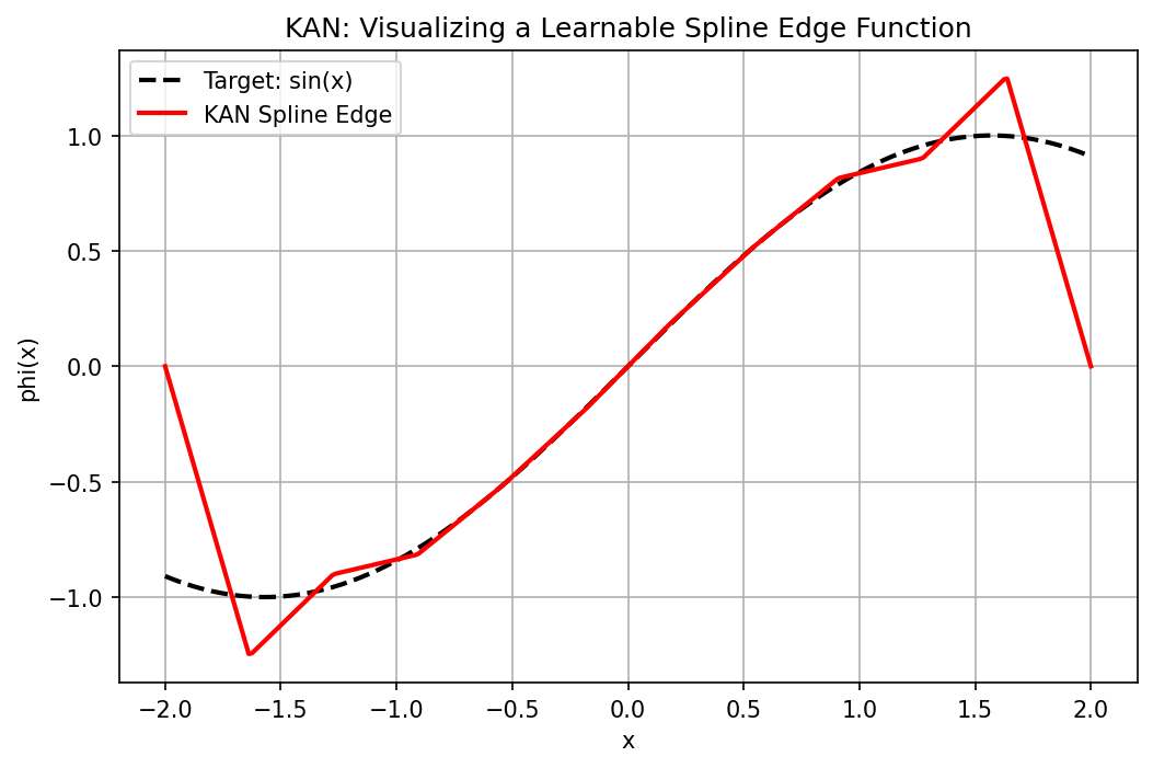
Demo 7.1: Visualizing a Learnable Spline Edge¶

Python

import matplotlib
matplotlib.use('Agg')
import torch
import torch.nn as nn
import numpy as np
import matplotlib.pyplot as plt

# Simplified B-spline implementation using piecewise linear basis
def b_spline_basis(x, knots):
    """Piecewise linear B-spline basis over given knots."""
    n = len(knots) - 2
    bases = []
    for i in range(n):
        t0, t1, t2 = knots[i], knots[i+1], knots[i+2]
        left  = torch.clamp((x - t0) / (t1 - t0 + 1e-8), 0.0, 1.0)
        right = torch.clamp((t2 - x) / (t2 - t1 + 1e-8), 0.0, 1.0)
        bases.append(torch.min(left, right))
    return torch.stack(bases, dim=-1)  # shape: (N, n)

class KANLayer(nn.Module):
    def __init__(self, in_dim, out_dim, G=10):
        super().__init__()
        self.in_dim = in_dim
        self.out_dim = out_dim
        self.G = G
        # Learnable control points: one set per (in, out) pair
        self.phi = nn.Parameter(torch.randn(in_dim, out_dim, G))
        knots_raw = torch.linspace(-2, 2, G + 2)
        self.register_buffer('knots', knots_raw)

    def forward(self, x):
        # x: (batch, in_dim)
        outs = []
        for i in range(self.in_dim):
            xi = x[:, i]  # (batch,)
            basis = b_spline_basis(xi, self.knots)  # (batch, G)
            # For each output dimension, compute weighted sum
            col = (basis.unsqueeze(1) * self.phi[i].unsqueeze(0)).sum(-1)  # (batch, out_dim)
            outs.append(col)
        return torch.stack(outs, dim=0).sum(0)  # (batch, out_dim)

# Instantiate and visualize
torch.manual_seed(42)
layer = KANLayer(in_dim=1, out_dim=1, G=10)

# Train to approximate sin(x) on [-2, 2]
x_train = torch.linspace(-2, 2, 200).unsqueeze(1)
y_train = torch.sin(x_train)

opt = torch.optim.Adam(layer.parameters(), lr=0.05)
for _ in range(1000):
    opt.zero_grad()
    loss = nn.MSELoss()(layer(x_train), y_train)
    loss.backward()
    opt.step()

print(f"Final MSE: {loss.item():.6f}")

# Visualize the learned edge function
x_vis = torch.linspace(-2, 2, 300).unsqueeze(1)
with torch.no_grad():
    y_pred = layer(x_vis).squeeze().numpy()
    y_true = torch.sin(x_vis).squeeze().numpy()

plt.figure(figsize=(8, 5))
plt.plot(x_vis.squeeze().numpy(), y_true, 'k--', linewidth=2, label='Target: sin(x)')
plt.plot(x_vis.squeeze().numpy(), y_pred, 'r-', linewidth=2, label='KAN Spline Edge')
plt.title("KAN: Visualizing a Learnable Spline Edge Function")
plt.xlabel("x"); plt.ylabel("phi(x)")
plt.legend(); plt.grid(True)
plt.savefig('figures/02-4-demo1.png', dpi=150, bbox_inches='tight')
plt.close()

Text Only

Final MSE: 0.048438

Demo 7.2: Symbolic Regression with pykan¶

(Note: Requires pykan library)