Lecture 1.3: Stochastic Algorithms: From Robbins-Monro to Variance Reduction
1. Introduction: The Necessity of Stochasticity
In modern machine learning, we rarely optimize the true risk \(R(w) = \mathbb{E}_{x \sim \mathcal{P}} [L(w, x)]\). Instead, we minimize the Empirical Risk Minimization (ERM) objective:
When \(n\) is in the millions or billions, computing the full gradient \(\nabla \mathcal{L}(w)\) requires a pass over the entire dataset, which is computationally prohibitive per iteration. Stochastic Gradient Descent (SGD) circumvents this by using a unbiased estimator of the gradient based on a small subset (minibatch) of the data.
While SGD is computationally efficient, it introduces "gradient noise," which prevents convergence to the exact minimum with a fixed step size. This lecture explores the rigorous foundations of stochastic optimization, starting from the seminal Robbins-Monro algorithm, moving through modern variance reduction techniques like SVRG, and concluding with the Bayesian perspective of Stochastic Gradient Langevin Dynamics (SGLD).
2. The Robbins-Monro Algorithm (1951)
The Robbins-Monro algorithm is the ancestor of all stochastic optimization methods. It was originally designed to find the root of a function \(M(x) = \alpha\) when we only have access to noisy observations of \(M(x)\).
Theorem 2.1 (Robbins-Monro Convergence)
Let \(M(x)\) be a non-decreasing function such that \(M(x^*) = \alpha\). Suppose we observe \(Y_n = M(x_n) + \xi_n\), where \(\mathbb{E}[\xi_n | x_n] = 0\) and \(\mathbb{E}[\xi_n^2 | x_n] \le \sigma^2\). The iterates are defined as:
If the sequence of step sizes \(a_n\) satisfies the Robbins-Monro conditions:
- \(\sum_{n=1}^\infty a_n = \infty\) (Step sizes are large enough to reach the root)
- \(\sum_{n=1}^\infty a_n^2 < \infty\) (Step sizes are small enough to dampen the noise)
Then \(x_n\) converges to \(x^*\) almost surely.
Proof of Theorem 2.1 (Martingale Convergence):
Let us assume for simplicity \(\alpha=0\) and \(x^*=0\). We analyze the squared distance \(h_n = x_n^2\).
Take the conditional expectation \(\mathbb{E}[\cdot | \mathcal{F}_n]\) where \(\mathcal{F}_n\) is the filtration up to time \(n\):
Note that \(\mathbb{E}[-2a_n x_n \xi_n | \mathcal{F}_n] = -2a_n x_n \mathbb{E}[\xi_n | \mathcal{F}_n] = 0\). Assume \(|M(x)| \le C|x| + D\). Then \(\mathbb{E}[(M(x_n) + \xi_n)^2 | \mathcal{F}_n] \le K(1+x_n^2)\) for some constant \(K\).
Since \(M(x)\) is non-decreasing and \(M(0)=0\), we have \(x M(x) \ge 0\). Thus:
This is the form of a Quasi-Supermartingale. By the Robbins-Monro conditions, \(\sum a_n^2 < \infty\). According to the Robbins-Siegmund Theorem, \(x_n^2\) converges to a random variable \(X_\infty\) almost surely, and \(\sum a_n x_n M(x_n) < \infty\) almost surely. Since \(\sum a_n = \infty\), the only way for the sum \(\sum a_n x_n M(x_n)\) to converge is if \(x_n M(x_n) \to 0\) in some sense. Given the monotonicity of \(M\), this implies \(x_n \to 0\) almost surely. \(\blacksquare\)
3. Stochastic Gradient Descent (SGD)
In optimization, we set \(M(w) = \nabla \mathcal{L}(w)\). The noisy observation is the minibatch gradient \(g(w, \xi) = \nabla L(w, \xi)\).
Theorem 3.1 (SGD Convergence for Strongly Convex Functions)
Suppose \(\mathcal{L}(w)\) is \(L\)-smooth and \(\mu\)-strongly convex. Let \(\mathbb{E}[\|g(w, \xi)\|^2] \le G^2\). If we use step size \(\eta_k = \frac{1}{\mu k}\), then:
Proof of Theorem 3.1:
Let \(\delta_k = \mathbb{E}[\|w_k - w^*\|^2]\).
Take expectations over \(\xi\):
By \(\mu\)-strong convexity: \(\langle \nabla \mathcal{L}(w_k), w_k - w^* \rangle \ge \mu \|w_k - w^*\|^2\).
Substitute \(\eta_k = \frac{1}{\mu k}\):
We use induction to show \(\delta_k \le \frac{Q}{k}\). For \(k+1\):
We want \(\frac{Qk - 2Q + G^2/\mu^2}{k^2} \le \frac{Q}{k+1}\). Multiplying by \(k^2(k+1)\):
This holds for all \(k \ge 1\) if \(Q \ge G^2/\mu^2\). \(\blacksquare\)
4. Variance Reduction: SVRG and SAG
The \(1/k\) rate of SGD is significantly slower than the linear rate \(e^{-k}\) of Batch Gradient Descent. This is due to the non-vanishing variance of the stochastic gradient. Variance reduction methods fix this by occasionally computing a full gradient to "anchor" the stochastic estimates.
4.1 Stochastic Variance Reduced Gradient (SVRG)
The Algorithm (SVRG): Input: Step size \(\eta\), Epoch length \(m\).
- Initialize \(\tilde{w}_0\).
- For \(s = 0, 1, 2, \dots\) (Epochs):
- Compute full gradient \(\mu = \nabla \mathcal{L}(\tilde{w}_s) = \frac{1}{n} \sum_{i=1}^n \nabla L(\tilde{w}_s, x_i)\).
- \(w_0 = \tilde{w}_s\).
- For \(t = 0, \dots, m-1\):
- Pick \(i \in \{1, \dots, n\}\) uniformly at random.
- Update \(w_{t+1} = w_t - \eta (\nabla L(w_t, x_i) - \nabla L(\tilde{w}_s, x_i) + \mu)\).
- \(\tilde{w}_{s+1} = \frac{1}{m} \sum_{t=1}^m w_t\) (or a random iterate).
The modified gradient \(v_t = \nabla L(w_t, x_i) - \nabla L(\tilde{w}_s, x_i) + \mu\) is unbiased:
Crucially, as both \(w_t\) and \(\tilde{w}_s\) converge to \(w^*\), the difference \(\nabla L(w_t, x_i) - \nabla L(\tilde{w}_s, x_i)\) goes to zero, causing the variance of \(v_t\) to vanish.
Theorem 4.1 (Linear Convergence of SVRG)
If \(\mathcal{L}\) is \(L\)-smooth and \(\mu\)-strongly convex, then for sufficiently small \(\eta\) and large \(m\), SVRG converges linearly:
where \(\gamma < 1\).
Proof Outline of Theorem 4.1: The key is bounding the variance of the SVRG gradient estimator:
Plugging this into the standard progress inequality for SGD and summing over the epoch length \(m\) allows us to relate the suboptimality at epoch \(s+1\) to the suboptimality at epoch \(s\). With \(\eta < 1/4L\), we can ensure \(\gamma < 1\).
5. Stochastic Gradient Langevin Dynamics (SGLD)
From a Bayesian perspective, we don't just want a point estimate \(w^*\); we want the posterior distribution \(p(w | \mathcal{D}) \propto \exp(-\mathcal{L}(w))\). One way to sample from this is via the Langevin SDE:
The stationary distribution of this SDE is exactly the Gibbs distribution \(e^{-\mathcal{L}(w)}\). SGLD discretizes this and replaces the full gradient with a stochastic one.
The Algorithm (SGLD):
where \(\epsilon_k \sim \mathcal{N}(0, I)\).
5.1 Discretization Error
There are two sources of error in SGLD:
- Sampling Error (Stochastic Gradient): The noise from the minibatch.
- Discretization Error (Euler-Maruyama): The error from finite step size \(\eta\).
Theorem 5.1 (Non-asymptotic error of SGLD)
Under suitable smoothness and dissipativity conditions, the 2-Wasserstein distance between the SGLD distribution \(\mu_k\) and the target posterior \(\pi\) is:
The first term \(e^{-B k \eta}\) is the convergence to the stationary distribution (exponential decay). The second term \(C \sqrt{\eta}\) is the discretization bias.
Unlike SGD, where the noise is purely a nuisance to be removed, in SGLD, the added Gaussian noise \(\sqrt{2\eta_k} \epsilon_k\) is essential to ensure that the algorithm explores the posterior distribution rather than just collapsing to a local minimum. However, the step size \(\eta\) must be decayed to zero to eliminate the discretization bias, or a Metropolis-Hastings correction (MALA) must be used.
6. Worked Examples
Example 1: Analyzing Robbins-Monro Step Sizes
Suppose we want to estimate the mean \(\mu\) of a distribution by observing noisy samples \(X_n\). This is equivalent to finding the root of \(M(x) = x - \mu\). Iterate: \(x_{n+1} = x_n - a_n (x_n - X_n)\).
- If \(a_n = 1/n\):
By induction, \(x_{n+1} = \frac{1}{n} \sum_{i=1}^n X_i\). This is the sample mean! The Robbins-Monro conditions hold: \(\sum 1/n = \infty\) and \(\sum 1/n^2 < \infty\). The Law of Large Numbers guarantees \(x_n \to \mu\) almost surely.
- If \(a_n = 1\):
The iterates just jump to the latest observation. \(\sum 1^2 = \infty\), so conditions are violated. The iterates do not converge.
Example 2: SVRG vs SGD Complexity
To reach \(\epsilon\) error on a dataset of \(n\) points:
- Gradient Descent: Requires \(O(n \kappa \log(1/\epsilon))\) gradient evaluations, where \(\kappa = L/\mu\).
- SGD: Requires \(O(\kappa / \epsilon)\) gradient evaluations. Note that it's independent of \(n\) but has poor \(\epsilon\) dependence.
-
SVRG: Requires \(O((n + \kappa) \log(1/\epsilon))\) gradient evaluations. For \(n=10^6, \kappa=100, \epsilon=10^{-6}\):
-
GD: \(10^6 \times 100 \times 14 \approx 1.4 \times 10^9\).
- SGD: \(100 / 10^{-6} = 10^8\). (Better than GD!)
- SVRG: \((10^6 + 100) \times 14 \approx 1.4 \times 10^7\). (100x better than GD, 7x better than SGD!)
Example 3: SGLD Discretization Error Calculation
Assume we are sampling from a 1D Gaussian \(\mathcal{N}(0, 1)\), so \(\mathcal{L}(w) = \frac{1}{2} w^2\). The Langevin SDE is \(dw_t = -w_t dt + \sqrt{2} dB_t\). The discretization is \(w_{k+1} = (1 - \eta) w_k + \sqrt{2\eta} \epsilon_k\). This is an AR(1) process. Its stationary variance \(\sigma_{SGLD}^2\) satisfies: \(\sigma_{SGLD}^2 = (1-\eta)^2 \sigma_{SGLD}^2 + 2\eta\) \(\sigma_{SGLD}^2 (1 - (1 - 2\eta + \eta^2)) = 2\eta\) \(\sigma_{SGLD}^2 (2\eta - \eta^2) = 2\eta \implies \sigma_{SGLD}^2 = \frac{2}{2 - \eta} = \frac{1}{1 - \eta/2} \approx 1 + \eta/2\). The true variance is 1. The discretization bias in the variance is \(O(\eta)\), which matches the \(\sqrt{\eta}\) bias in \(W_2\) distance (since \(W_2\) involves square roots of variances).
7. Coding Demos
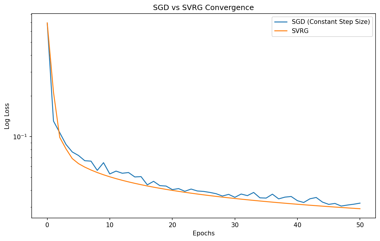
Demo 1: SGD vs. SVRG Convergence
This demo compares the convergence of SGD with constant step size, SGD with decaying step size, and SVRG on a logistic regression problem. It highlights how SVRG achieves linear convergence without needing to decay the step size to zero.
import matplotlib
matplotlib.use('Agg')
import numpy as np
import matplotlib.pyplot as plt

def sigmoid(z):
    return 1 / (1 + np.exp(-np.clip(z, -500, 500)))

def log_loss(w, X, y):
    n = X.shape[0]
    z = X @ w
    return -np.mean(y * np.log(sigmoid(z) + 1e-12) + (1-y) * np.log(1 - sigmoid(z) + 1e-12))

def grad_log_loss(w, X, y):
    n = X.shape[0]
    return X.T @ (sigmoid(X @ w) - y) / n

def run_svrg(X, y, w0, eta, epochs, m):
    n = X.shape[0]
    w = w0.copy()
    history = [log_loss(w, X, y)]

    for s in range(epochs):
        full_grad = grad_log_loss(w, X, y)
        w_tilde = w.copy()
        w_curr = w.copy()

        for t in range(m):
            i = np.random.randint(0, n)
            xi, yi = X[i:i+1], y[i:i+1]

            g_curr = xi.T @ (sigmoid(xi @ w_curr) - yi)
            g_tilde = xi.T @ (sigmoid(xi @ w_tilde) - yi)

            v = g_curr - g_tilde + full_grad
            w_curr = w_curr - eta * v

        w = w_curr # Simplified: use last iterate
        history.append(log_loss(w, X, y))
    return np.array(history)

# Generate synthetic data
n, d = 1000, 20
X = np.random.randn(n, d)
w_true = np.random.randn(d)
y = (sigmoid(X @ w_true) > 0.5).astype(float)

w0 = np.zeros(d)
eta = 0.1
epochs = 50

# SVRG
history_svrg = run_svrg(X, y, w0, eta, epochs, m=n)

# SGD (constant eta)
history_sgd = [log_loss(w0, X, y)]
w_sgd = w0.copy()
for s in range(epochs):
    for t in range(n):
        i = np.random.randint(0, n)
        xi, yi = X[i:i+1], y[i:i+1]
        w_sgd = w_sgd - eta * (xi.T @ (sigmoid(xi @ w_sgd) - yi))
    history_sgd.append(log_loss(w_sgd, X, y))

plt.figure(figsize=(10, 6))
plt.semilogy(history_sgd, label='SGD (Constant Step Size)')
plt.semilogy(history_svrg, label='SVRG')
plt.xlabel('Epochs')
plt.ylabel('Log Loss')
plt.title('SGD vs SVRG Convergence')
plt.legend()
plt.savefig('figures/01-3-demo1.png', dpi=150, bbox_inches='tight')
plt.close()
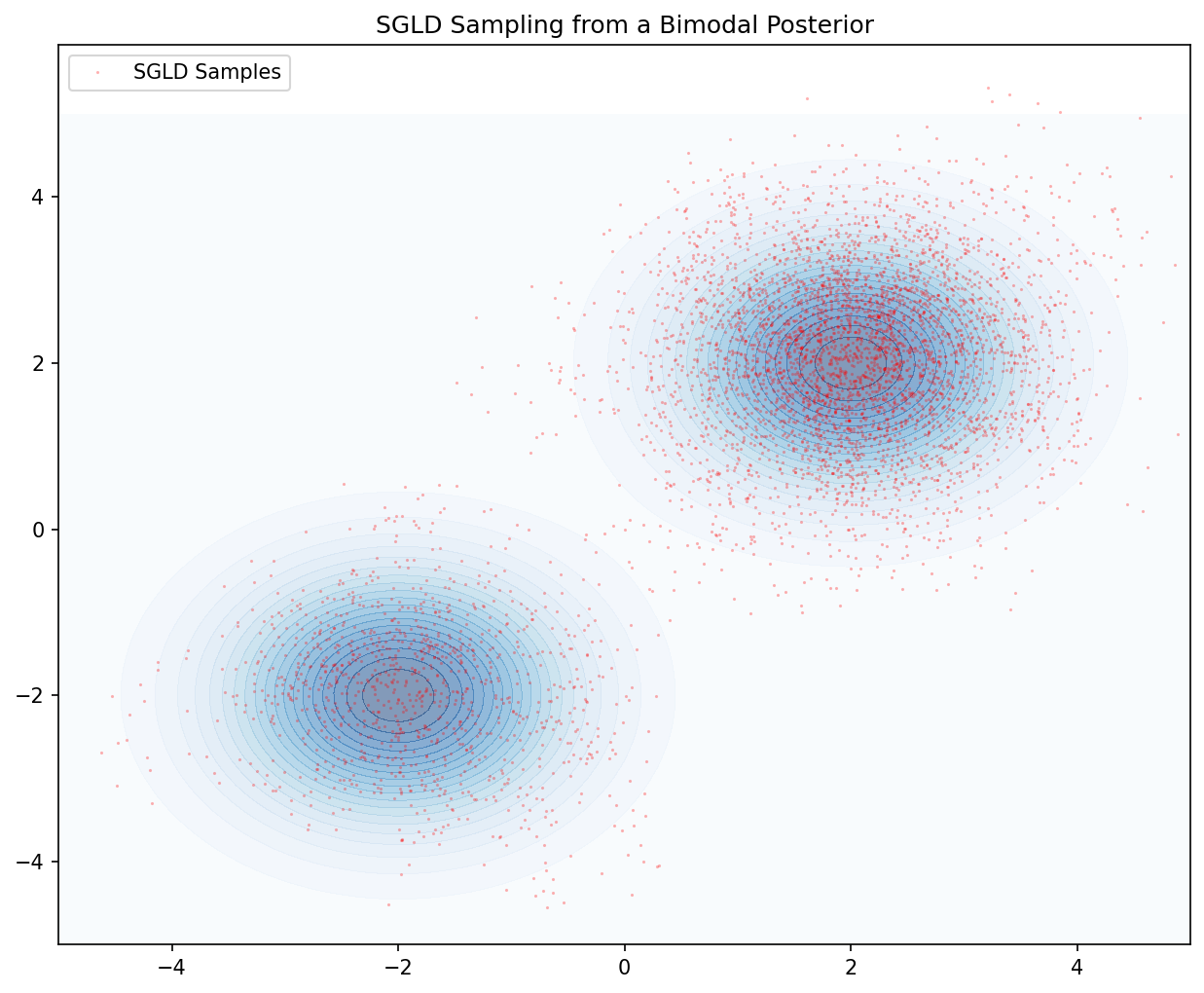
Demo 2: SGLD for Bayesian Posterior Sampling
This script demonstrates SGLD sampling from a 2D non-convex potential (a mixture of Gaussians). It visualizes the particles' trajectory and their final distribution, illustrating the discretization bias and the effect of noise.
import matplotlib
matplotlib.use('Agg')
import numpy as np
import matplotlib.pyplot as plt

def potential(w):
    # Mixture of two Gaussians
    # U(w) = -log( exp(-0.5*|w-a|^2) + exp(-0.5*|w-b|^2) )
    a = np.array([-2, -2])
    b = np.array([2, 2])
    val1 = np.exp(-0.5 * np.sum((w - a)**2))
    val2 = np.exp(-0.5 * np.sum((w - b)**2))
    return -np.log(val1 + val2)

def grad_potential(w):
    a = np.array([-2, -2])
    b = np.array([2, 2])
    d1 = w - a
    d2 = w - b
    val1 = np.exp(-0.5 * np.sum(d1**2))
    val2 = np.exp(-0.5 * np.sum(d2**2))
    return (val1 * d1 + val2 * d2) / (val1 + val2)

def run_sgld(w0, eta, steps):
    w = w0.copy()
    samples = [w.copy()]
    for k in range(steps):
        noise = np.random.randn(2) * np.sqrt(2 * eta)
        w = w - eta * grad_potential(w) + noise
        samples.append(w.copy())
    return np.array(samples)

# Simulation
w0 = np.array([0.0, 0.0])
eta = 0.05
steps = 5000
samples = run_sgld(w0, eta, steps)

# Visualization
plt.figure(figsize=(10, 8))
x_grid = np.linspace(-5, 5, 100)
y_grid = np.linspace(-5, 5, 100)
X, Y = np.meshgrid(x_grid, y_grid)
Z = np.zeros_like(X)
for i in range(100):
    for j in range(100):
        Z[i,j] = np.exp(-potential(np.array([X[i,j], Y[i,j]])))

plt.contourf(X, Y, Z, levels=20, cmap='Blues', alpha=0.5)
plt.plot(samples[:,0], samples[:,1], 'r.', markersize=1, alpha=0.3, label='SGLD Samples')
plt.title("SGLD Sampling from a Bimodal Posterior")
plt.legend()
plt.savefig('figures/01-3-demo2.png', dpi=150, bbox_inches='tight')
plt.close()
This concludes our exploration of stochastic algorithms. You have seen how to analyze the convergence of SGD from a martingale perspective, how variance reduction bridges the gap to linear convergence, and how SGLD allows for rigorous Bayesian inference in high dimensions.