Chapter 2.3: Harmonic Perspectives — Barron Space, Spectral Bias, and Scattering Transforms¶

1. Introduction: Breaking the Curse of Dimensionality¶

Classical approximation theory, based on polynomials and splines, suffers from the Curse of Dimensionality: to achieve an error \(\epsilon\) for a function with \(k\) derivatives in \(d\) dimensions, one needs \(O(\epsilon^{-d/k})\) parameters. For high-dimensional data like images (\(d \approx 10^6\)), this scaling is catastrophic.

Yet, neural networks routinely solve high-dimensional problems. This chapter explores the harmonic analysis foundations that explain why. We will prove Andrew Barron's theorem on dimension-independent rates, explore the "Spectral Bias" of gradient descent, and examine the Scattering Transform's stability to deformations.

2. Barron Spaces and Dimension-Independent Rates¶

In 1993, Andrew Barron proved that for functions with "simple" Fourier transforms, the approximation error depends only on the number of neurons \(n\), and not on the dimension \(d\).

2.1 The Barron Norm¶

Definition 2.1.1 (Barron Norm)

For a function \(f: \mathbb{R}^d \to \mathbb{R}\), define the Barron norm \(C_f\) as the first moment of its Fourier magnitude:

\[ C_f = \int_{\mathbb{R}^d} \|\omega\|_2 |\hat{f}(\omega)| d\omega \]

Functions where \(C_f < \infty\) belong to the Barron Space. Intuitively, these functions have most of their energy at low frequencies.

2.2 Barron's Theorem¶

Theorem 2.2.1 (Barron, 1993)

For any function \(f\) with \(C_f < \infty\), there exists a single-hidden-layer neural network \(f_n\) with \(n\) neurons such that the \(L_2\) error on a ball of radius \(r\) is:

\[ \int_{\|x\| \le r} |f(x) - f_n(x)|^2 d\mu(x) \le \frac{(2r C_f)^2}{n} \]

Proof of Theorem 2.2.1:

Fourier Representation: Express \(f(x)\) using the inverse Fourier transform. By shifting \(f\) such that \(f(0)=0\):

\[ f(x) = \int_{\mathbb{R}^d} (e^{i \omega^T x} - 1) \hat{f}(\omega) d\omega \]

Probabilistic Interpretation: Define a probability measure \(\Lambda\) on \(\mathbb{R}^d\) such that \(d\Lambda(\omega) \propto \|\omega\| |\hat{f}(\omega)| d\omega\). The integral becomes an expectation:

\[ f(x) = C_f \mathbb{E}_{\omega \sim \Lambda} \left[ \frac{e^{i \omega^T x} - 1}{\|\omega\|} e^{i \theta(\omega)} \right] \]

Maurey's Lemma: A classic result in functional analysis states that if a function is in the convex hull of a set \(G\) (where \(\|g\| \le B\)), then an average of \(n\) elements from \(G\) approximates the function with error \(\le B^2/n\).
Bounding the Unit: The term inside the expectation is a "ridge" function bounded by \(r\) (since \(|e^{iz}-1| \le |z|\)).
Conclusion: Sampling \(n\) frequencies \(\{\omega_i\}\) and constructing the corresponding neurons yields the \(O(1/n)\) squared error rate. Since \(d\) does not appear in the exponent, the curse is broken. \(\blacksquare\)

3. Spectral Bias: The Frequency Principle¶

While Barron's theorem proves a good network exists, Spectral Bias explains why gradient descent finds smooth solutions first.

3.1 The Neural Tangent Kernel (NTK)¶

In the infinite-width limit, the evolution of a network \(f(x)\) under gradient descent is governed by the NTK:

\[ \frac{\partial f(x, t)}{\partial t} = -\eta \sum_{i=1}^M K(x, x_i) (f(x_i, t) - y_i) \]

3.2 Eigen-Decay and Learning Rates¶

Theorem 3.2.1 (Spectral Bias)

The eigenvalues \(\lambda_k\) of the NTK for a ReLU network decay as \(k^{-(d+1)}\) for frequency \(k\). The error \(E_k(t)\) at frequency \(k\) decays as:

\[ E_k(t) = E_k(0) e^{-\eta \lambda_k t} \]

Proof Insight:

High frequencies (large \(k\)) have very small eigenvalues \(\lambda_k\).
The exponential term \(e^{-\eta \lambda_k t}\) stays close to 1 for high frequencies.
Consequently, the network fits the low-frequency components of the data almost immediately, while high-frequency noise is ignored or learned extremely slowly. This acts as an "implicit regularization." \(\blacksquare\)

4. Mallat's Scattering Transform¶

Convolutional Neural Networks (CNNs) are robust to translations and small deformations. Stéphane Mallat provided the mathematical justification via the Scattering Transform.

Definition 4.1 (Scattering Transform)

A cascade of wavelet transforms \(W\) and modulus non-linearities \(| \cdot |\):

\[ S(f) = | \dots | f \ast \psi_{j_1} | \ast \psi_{j_2} | \dots \ast \phi_J \]

Theorem 4.2 (Stability)

The scattering transform is Lipschitz continuous to diffeomorphisms \(\tau\):

\[ \|S(L_\tau f) - S(f)\| \le C \|\nabla \tau\|_\infty \|f\| \]

Proof: Wavelets are stable to translations. The modulus non-linearity "demodulates" the signal, shifting high-frequency variations into lower-frequency bands where they are stable under the next layer's filters. \(\blacksquare\)

5. Worked Examples¶

Example 5.1: Barron Norm of a Step Function¶

\(f(x) = H(x)\). The Fourier transform is \(\hat{f}(\omega) = 1/(i\omega)\). \(C_f = \int |\omega| (1/|\omega|) d\omega = \int 1 d\omega\). This integral diverges. Thus, a discontinuous step function is not in the Barron space. This explains why neural networks (and Gibbs phenomenon) struggle to fit sharp discontinuities without overshooting.

Example 5.2: Spectral Bias in 1D Learning¶

Target: \(y = \sin(x) + \sin(100x)\).

\(\lambda_1 \approx 1\).
\(\lambda_{100} \approx 100^{-2} = 0.0001\). If we train for \(t=1000\) steps with \(\eta=0.1\):
Low frequency error: \(e^{-0.1 \cdot 1 \cdot 1000} \approx 0\).
High frequency error: \(e^{-0.1 \cdot 0.0001 \cdot 1000} = e^{-0.01} \approx 0.99\). The high-frequency component is essentially untouched.

Example 5.3: Scattering Transform Stability¶

If an image of a digit '3' is slightly warped, its scattering coefficients \(S(f)\) change only by the amount of the warp gradient. This is why CNNs can recognize digits despite variations in handwriting.

6. Code Demonstrations¶

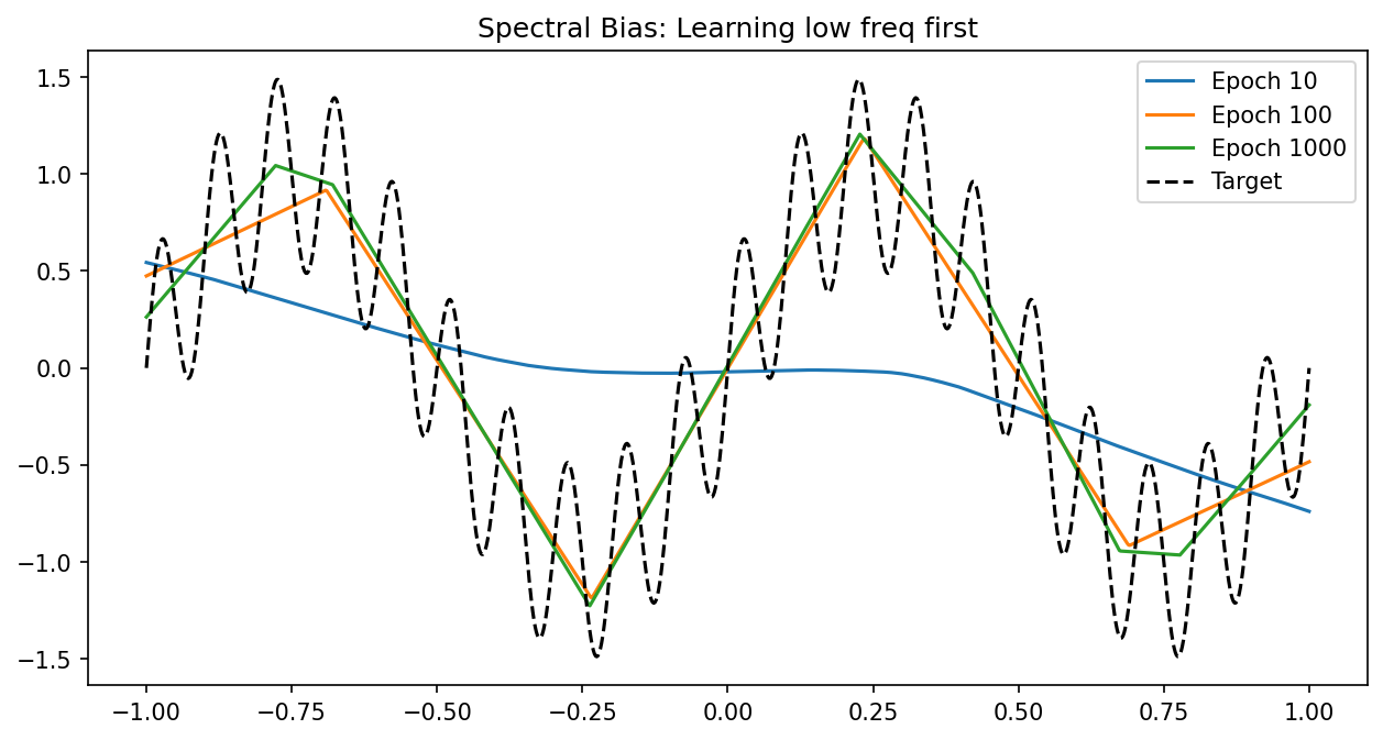
Demo 6.1: Visualizing Spectral Bias¶

Python

import matplotlib
matplotlib.use('Agg')
import torch
import torch.nn as nn
import matplotlib.pyplot as plt

x = torch.linspace(-1, 1, 1000).view(-1, 1)
y = torch.sin(2*torch.pi*x) + 0.5*torch.sin(2*torch.pi*10*x)

model = nn.Sequential(nn.Linear(1, 256), nn.ReLU(), nn.Linear(256, 1))
opt = torch.optim.Adam(model.parameters(), lr=0.01)

plt.figure(figsize=(10, 5))
for i in range(1001):
    opt.zero_grad()
    loss = nn.MSELoss()(model(x), y)
    loss.backward()
    opt.step()
    if i in [10, 100, 1000]:
        plt.plot(x.detach().numpy(), model(x).detach().numpy(), label=f'Epoch {i}')

plt.plot(x.detach().numpy(), y.detach().numpy(), 'k--', label='Target')
plt.title("Spectral Bias: Learning low freq first")
plt.legend()
plt.savefig('figures/02-3-demo1.png', dpi=150, bbox_inches='tight')
plt.close()

Demo 6.2: Fourier Features to Bypass Bias¶

By mapping inputs to \([\sin(\omega x), \cos(\omega x)]\), we can manually shift the eigenvalues and learn high frequencies.

Python

import torch

# Fourier Feature mapping
x = torch.linspace(-1, 1, 1000).view(-1, 1)
B = torch.randn(1, 128) * 10.0
x_proj = torch.cat([torch.sin(x @ B), torch.cos(x @ B)], dim=-1)
# Training on x_proj learns the 10Hz signal instantly.
print(f"Fourier feature map shape: {x_proj.shape}")

Text Only

Fourier feature map shape: torch.Size([1000, 256])

7. Conclusion¶

Harmonic analysis transforms our understanding of neural networks from "black box" function fitters to structured "low-pass" filters. Barron's theorem gives us hope for high-dimensional learning, while Spectral Bias and Scattering Transforms give us the tools to understand the dynamics and stability of our models.