Chapter 3.2: Complexity Measures and VC Theory
Generalization bounds via concentration inequalities (like McDiarmid's) require bounding the worst-case deviation between true risk and empirical risk uniformly over an entire hypothesis class. The fundamental challenge of learning theory is quantifying the "size" or "complexity" of these classes, particularly when they contain infinitely many functions (e.g., continuous parameter spaces in neural networks).
This chapter exhaustively details rigorous mathematical frameworks to measure complexity: the Vapnik-Chervonenkis (VC) dimension for binary classification, Rademacher Complexity for real-valued functions, and Dudley's Entropy Chaining Integral. We present meticulous proofs for the pivotal Sauer-Shelah lemma, metric entropy bounds, and chaining mechanics.
1. The Vapnik-Chervonenkis (VC) Dimension
The VC dimension fundamentally assesses how effectively a hypothesis class can separate, or "shatter," discrete datasets. It is a strictly combinatorial metric applied purely to binary classification functions mapping to \(\{0, 1\}\).
1.1 Growth Functions and Shattering
Definition 1.1 (Growth Function)
Let \(\mathcal{H}\) be a hypothesis class mapping an input space \(\mathcal{X}\) to \(\{0, 1\}\). For any specific set of \(n\) points \(C = \{x_1, \dots, x_n\} \subseteq \mathcal{X}\), the restriction of \(\mathcal{H}\) to \(C\) is the set of all unique binary vectors it generates:
The growth function \(\Pi_{\mathcal{H}}(n)\) is the maximum cardinality of this restricted set over all possible choices of \(n\) points:
Trivially, the growth function is bounded by the total number of binary assignments: \(\Pi_{\mathcal{H}}(n) \le 2^n\).
Definition 1.2 (Shattering and VC Dimension)
If \(\Pi_{\mathcal{H}}(n) = 2^n\), it means there exists at least one set of \(n\) points that \(\mathcal{H}\) can assign every possible combination of \(0\)s and \(1\)s. We say \(\mathcal{H}\) shatters this set. The VC dimension, denoted \(\text{VCdim}(\mathcal{H})\), is the maximum integer \(n\) such that \(\Pi_{\mathcal{H}}(n) = 2^n\). If the class can shatter arbitrarily large finite sets, the VC dimension is infinity.
1.2 The Sauer-Shelah Lemma
If the VC dimension is finite, say \(d\), the growth function does not just drop slightly below \(2^n\); it undergoes a dramatic phase transition, becoming bounded strictly by a polynomial of degree \(d\).
Theorem 1.3 (Sauer-Shelah Lemma)
Let \(\mathcal{H}\) be a hypothesis class with \(\text{VCdim}(\mathcal{H}) = d < \infty\). Then for any \(n\),
For \(n \ge d\), this sum is tightly bounded by \((\frac{en}{d})^d\).
Proof: We utilize induction on the parameters \(n\) and \(d\). Let the upper bound function be defined as \(g(n, d) = \sum_{i=0}^d \binom{n}{i}\). A fundamental identity of binomial coefficients (Pascal's Triangle) is \(g(n, d) = g(n-1, d) + g(n-1, d-1)\).
Base cases: If \(n = 0\), the maximum number of dichotomies over an empty set is \(1\). The sum evaluates to \(\binom{0}{0} = 1\), so \(g(0, d) = 1\). The bound holds. If \(d = 0\), the hypothesis class can only shatter sets of size \(0\), implying the class contains only a single constant function. Thus \(\Pi_{\mathcal{H}}(n) = 1\). The sum evaluates to \(\binom{n}{0} = 1 = g(n, 0)\). The bound holds.
Inductive step: Assume the lemma holds true for \((n-1, d)\) and \((n-1, d-1)\). We will prove it for \((n, d)\). Take any set \(C = \{x_1, \dots, x_n\}\). The restriction \(\mathcal{H}_C\) contains binary vectors of length \(n\). Define \(C' = \{x_1, \dots, x_{n-1}\}\), representing the first \(n-1\) points. We partition the dichotomies generated by \(\mathcal{H}_C\) into two constructed sets over \(C'\):
- \(S_1\) is the set of all unique prefixes of length \(n-1\) found in \(\mathcal{H}_C\). Note that \(|S_1| \le \Pi_{\mathcal{H}}(n-1)\).
- \(S_2\) is the subset of prefixes in \(S_1\) that exist in \(\mathcal{H}_C\) with both a \(0\) and a \(1\) appended at the \(n\)-th position. In other words, \(v \in S_2 \iff (v, 0) \in \mathcal{H}_C \text{ and } (v, 1) \in \mathcal{H}_C\).
Because every vector in \(\mathcal{H}_C\) either shares its prefix uniquely or shares it with exactly one other vector that differs only in the final coordinate, the total number of vectors is strictly the sum of unique prefixes plus the number of duplicated prefixes:
Because \(S_1\) is simply the projection of \(\mathcal{H}\) onto a set of \(n-1\) points, its VC dimension cannot exceed that of \(\mathcal{H}\), which is \(d\). By the inductive hypothesis:
Now, consider \(S_2\). We assert that the VC dimension of \(S_2\) is strictly bounded by \(d-1\). Suppose, by contradiction, that \(S_2\) shatters a subset \(A \subseteq C'\) of size \(d\). This means that for every possible binary pattern on \(A\), there exists a prefix \(v \in S_2\) matching that pattern. However, by the exact definition of \(S_2\), every vector \(v \in S_2\) can be appended with either a \(0\) or a \(1\) to form a valid dichotomy in \(\mathcal{H}_C\). This implies that \(\mathcal{H}_C\) can shatter the set \(A \cup \{x_n\}\), which is a set of size \(d+1\). But this directly violates the premise that \(\text{VCdim}(\mathcal{H}) = d\). Therefore, the largest set \(S_2\) can shatter is size \(d-1\). By the inductive hypothesis:
Combining these bounds via Pascal's identity completes the combinatorial leap:
Because this is true for any set \(C\), it bounds the global growth function. The bound \((\frac{en}{d})^d\) is a standard algebraic simplification. \(\blacksquare\)
1.3 The Fundamental Theorem of PAC Learning
By replacing the infinite complexity of \(\mathcal{H}\) with the finite bounded growth function over a sample, we derive universal convergence bounds.
Theorem 1.4 (VC Generalization Bound)
For a hypothesis class with finite VC dimension \(d\), with probability at least \(1-\delta\):
Proof Structure: The rigorous proof utilizes Vapnik and Chervonenkis's "Double Sample Trick". We introduce a hypothetical "ghost sample" \(S'\) of size \(n\). One proves that the probability of the empirical risk diverging from the true risk by \(t\) is strictly bounded by twice the probability of the empirical risk diverging from the empirical risk of the ghost sample by \(t/2\). We then condition heavily on the combined sample \(S \cup S'\) of size \(2n\). Over these fixed points, the infinite class \(\mathcal{H}\) acts identically to a finite class of size \(\Pi_{\mathcal{H}}(2n) \le (2en/d)^d\). We apply Hoeffding's inequality for a fixed hypothesis, and then apply the union bound strictly over this finite effective class. Solving the resulting algebraic inequality for the threshold yields the bound. \(\blacksquare\)
2. Rademacher Complexity
While the VC dimension perfectly characterizes binary classifiers, it collapses when dealing with continuous neural network outputs, regression, or probabilistic confidence scores. Rademacher complexity solves this by empirically measuring the capacity of a function class to fit random noise.
2.1 Empirical and Expected Rademacher Complexity
Definition 2.1 (Rademacher Variables and Complexity)
Let \(\mathcal{F}\) be a class of real-valued functions mapping \(\mathcal{X} \to \mathbb{R}\). Given a fixed sample dataset \(S = (x_1, \dots, x_n)\), we draw \(n\) independent Rademacher variables \(\sigma_1, \dots, \sigma_n\) where \(\mathbb{P}(\sigma_i = 1) = \mathbb{P}(\sigma_i = -1) = 0.5\). The empirical Rademacher complexity of \(\mathcal{F}\) on \(S\) is defined as the expectation over the random signs:
The true expected Rademacher complexity is the expectation over the sample data distribution:
Conceptually, the sum \(\sum \sigma_i f(x_i)\) is high if the function class contains a function \(f\) that can closely align with the random noise vector \(\sigma\). High complexity implies high capacity to memorize noise.
2.2 Rademacher Generalization Bound
Theorem 2.2 (Generalization via Rademacher)
Let the function class \(\mathcal{F}\) be bounded such that \(f(x) \in [0, 1]\) universally. Then for any \(\delta > 0\), with probability at least \(1-\delta\) over the draw of \(S\):
Proof: We begin by defining the exact worst-case uniform deviation random variable:
We establish concentration for \(\Phi(S)\) around its mean using McDiarmid's Inequality. If we swap a single data point \(x_i\) for \(x_i'\) to create \(S'\), the empirical mean \(\hat{\mathbb{E}}_S[f] = \frac{1}{n}\sum f(x_j)\) shifts by exactly \((f(x_i) - f(x_i'))/n\). Because \(f\) is strictly bounded in \([0,1]\), the maximum change is bounded by \(c_i = 1/n\). McDiarmid's Inequality thus guarantees:
Setting the exponential bound to \(\delta\) confirms that \(\Phi(S) \le \mathbb{E}_{S}[\Phi(S)] + \sqrt{\frac{\log(1/\delta)}{2n}}\) with probability \(1-\delta\). The rigorous challenge remains to bound the expectation \(\mathbb{E}_{S}[\Phi(S)]\) utilizing Rademacher complexity. We introduce a ghost sample \(S' = (x_1', \dots, x_n')\) drawn identically and independently. The true expectation \(\mathbb{E}[f]\) can be written exactly as the expectation of the empirical mean over the ghost sample \(\mathbb{E}_{S'}[\hat{\mathbb{E}}_{S'}[f]]\). Substituting this yields:
Because the supremum of an expectation is bounded by the expectation of the supremum (Jensen's inequality applied to the convex supremum operator), we extract the expectation:
Here lies the brilliant symmetrization step. Because \(x_i\) and \(x_i'\) are independent samples from the exact same distribution, the distribution of their difference \((f(x_i') - f(x_i))\) is perfectly symmetric around zero. Multiplying this difference by a random sign variable \(\sigma_i \in \{-1, 1\}\) does not alter its distribution whatsoever. We introduce the Rademacher variables \(\sigma\):
By the subadditivity of the supremum (\(\sup(A+B) \le \sup A + \sup B\)):
Because \(\sigma_i\) and \(-\sigma_i\) possess identical distributions, the two terms are functionally identical, strictly summing to \(2 \mathcal{R}_n(\mathcal{F})\). Substituting this upper bound into our concentrated McDiarmid bound concludes the proof rigorously. \(\blacksquare\)
3. Metric Entropy and Dudley's Chaining Integral
Calculating Rademacher complexity directly is difficult because taking a supremum over an infinite class of continuous functions is computationally intractable. We solve this geometrically using Metric Entropy and Chaining.
3.1 Covering Numbers and Metric Entropy
Definition 3.1 (Covering Number)
Given a metric space \((\mathcal{F}, d)\), an \(\epsilon\)-cover is a finite subset \(C \subseteq \mathcal{F}\) such that for every \(f \in \mathcal{F}\), there exists some \(c \in C\) where the distance \(d(f, c) \le \epsilon\). The covering number \(\mathcal{N}(\epsilon, \mathcal{F}, d)\) is the absolute minimum cardinality of any \(\epsilon\)-cover. The natural logarithm \(\log \mathcal{N}(\epsilon, \mathcal{F}, d)\) is defined as the Metric Entropy.
If we naively apply Massart's finite lemma to a single \(\epsilon\)-cover to bound Rademacher complexity, we incur a harsh additive penalty of exactly \(\epsilon\), ruining convergence rates. Dudley bypassed this entirely by architecting an infinite telescoping sum of progressively finer covers.
3.2 Dudley's Entropy Integral
Theorem 3.2 (Dudley's Chaining Integral)
Let \(\mathcal{F}\) be a function class mapping to the reals. Using the empirical \(L_2\) norm metric on the sample \(S\), defined as \(\|f - g\|_n = \sqrt{\frac{1}{n} \sum (f(x_i) - g(x_i))^2}\), the empirical Rademacher complexity is rigorously bounded by:
Proof: Without loss of generality, assume the zero function \(0 \in \mathcal{F}\). Let \(D\) represent the geometric diameter of the class under the empirical norm. We dynamically construct an infinite sequence of covers \(C_0, C_1, C_2, \dots\) at exponentially decaying granularities. Let \(\epsilon_k = 2^{-k} D\). Define \(C_k\) to be the minimal \(\epsilon_k\)-cover of \(\mathcal{F}\). The number of elements in \(C_k\) is precisely \(\mathcal{N}(\epsilon_k)\). For any specific target function \(f \in \mathcal{F}\), define its projection \(f_k \in C_k\) as the element in the \(k\)-th cover minimizing distance to \(f\). By definition, \(\|f - f_k\|_n \le \epsilon_k\). As \(k \to \infty\), the granularity \(\epsilon_k \to 0\), meaning the sequence \(f_k\) converges uniformly to \(f\). Because \(f_0 = 0\) (the 0th cover consists of a single point at the origin since its radius spans the whole space), we can express \(f\) perfectly as an infinite telescoping series:
We inject this series directly into the empirical Rademacher complexity formula:
By swapping the sum and bounding the supremum of sums strictly by the sum of suprema:
Let the difference function be denoted \(g_k = f_k - f_{k-1}\). We must rigorously bound the magnitude of \(g_k\). By the triangle inequality:
Since the sequence decays by halves (\(\epsilon_{k-1} = 2 \epsilon_k\)), we have \(\|g_k\|_n \le 3 \epsilon_k\). Critically, how many distinct difference functions \(g_k\) exist? Since \(f_k\) belongs to a set of size \(|C_k|\) and \(f_{k-1}\) belongs to a set of size \(|C_{k-1}|\), the maximum possible number of pairing combinations is strictly bounded by \(|C_k| \times |C_{k-1}| \le |C_k|^2\). We now hold a finite set of difference functions. Applying Massart's Finite Lemma (which states the expected supremum of \(M\) sub-Gaussian variables with variance \(\sigma^2/n\) is bounded by \(\sigma \sqrt{2 \log M / n}\)):
Summing this bound across the infinite series \(k=1 \dots \infty\):
We seamlessly translate this discrete series into a continuous integral. Because \(\epsilon_k = 2(\epsilon_k - \epsilon_{k+1})\), we can interpret the term \(2 \epsilon_k\) as representing an integral over a rectangular segment bounded by the decreasing step sizes. Bounding the discrete Riemann sum with the continuous integration operator yields an absolute constant factor, arriving at Dudley's finalized formulation:
This completes the majestic proof of chaining. \(\blacksquare\)
4. Worked Examples
Example 1: VC Dimension Verification of Linear Hyperplanes
Let \(\mathcal{H}\) be linear half-spaces in \(\mathbb{R}^d\), defined by \(h(x) = \text{sign}(w \cdot x + b)\). Lower Bound: We prove \(\text{VCdim} \ge d+1\) by shattering a specific simplex. Select the origin \(0\) and the standard basis vectors \(e_1, \dots, e_d\). For any binary label assignment vector \(y \in \{-1, 1\}^{d+1}\), we simply set the hyperplane weights identically to \(w = (y_1, \dots, y_d)\) and strategically position the bias \(b\) to correctly classify the origin point \(y_0\). This set of \(d+1\) points is consistently shattered. Upper Bound: We prove \(\text{VCdim} < d+2\). Consider any arbitrary set of \(d+2\) points. By Radon's geometric Theorem, any \(d+2\) points in \(\mathbb{R}^d\) must be partitionable into two strictly disjoint subsets \(A\) and \(B\) whose convex hulls geometrically intersect. If a linear hyperplane were to perfectly assign \(+1\) to set \(A\) and \(-1\) to set \(B\), it must linearly separate their convex hulls. Because the hulls intersect, such a hyperplane mathematically cannot exist. Thus, no set of \(d+2\) points can be shattered. Conclusion: \(\text{VCdim}(\mathcal{H}) = d+1\). The VC generalization bound confirms learning requires \(n = \mathcal{O}(d/\epsilon^2)\) samples.
Example 2: Rademacher Complexity of Sparse L1 Models
Analyze a linear hypothesis class structurally constrained by the \(L_1\) norm: \(f(x) = w \cdot x\), subject strictly to \(\|w\|_1 \le B\) and inputs bounded by \(\|x\|_\infty \le X_\infty\). Applying the definition:
Leveraging Holder's Inequality defining the dual relationship between \(L_1\) and \(L_\infty\) norms, the dot product is rigidly bounded by the product of norms:
Substituting the bounded supremum constraint \(\|w\|_1 \le B\) pulls it outside the expectation:
The \(L_\infty\) norm evaluates the absolute maximum over the \(d\) coordinates. Using Massart's finite lemma specifically on the set of \(2d\) vector coordinate bounds (positive and negative signs for absolute value), the expectation resolves to bounded sub-Gaussian deviations scaling logarithmically with dimension:
This establishes the monumental theoretical foundation that \(L_1\) regularization completely nullifies the curse of dimensionality, enabling successful machine learning in spaces where dimension scales exponentially beyond the sample size.
Example 3: Unifying VC Dimension via Dudley's Integral
Dudley's Integral acts as a universal bridge, effortlessly deriving VC dimension bounds using metric entropy. David Haussler proved geometrically that the covering number of any discrete VC class is strictly bounded: \(\mathcal{N}(\epsilon, \mathcal{H}, L_2) \le C (1/\epsilon)^{2d}\), where \(d\) is the VC dimension. Substituting this exponential relationship directly into Dudley's formula:
The internal integral evaluates strictly to a converging finite universal constant (\(\approx \sqrt{\pi}/2\)). Consequently, the full integration resolves precisely to \(\mathcal{O}(\sqrt{d/n})\). Dudley's chaining perfectly replicates the fundamental VC theorem, unifying discrete and continuous complexity measures.
5. Coding Demonstrations
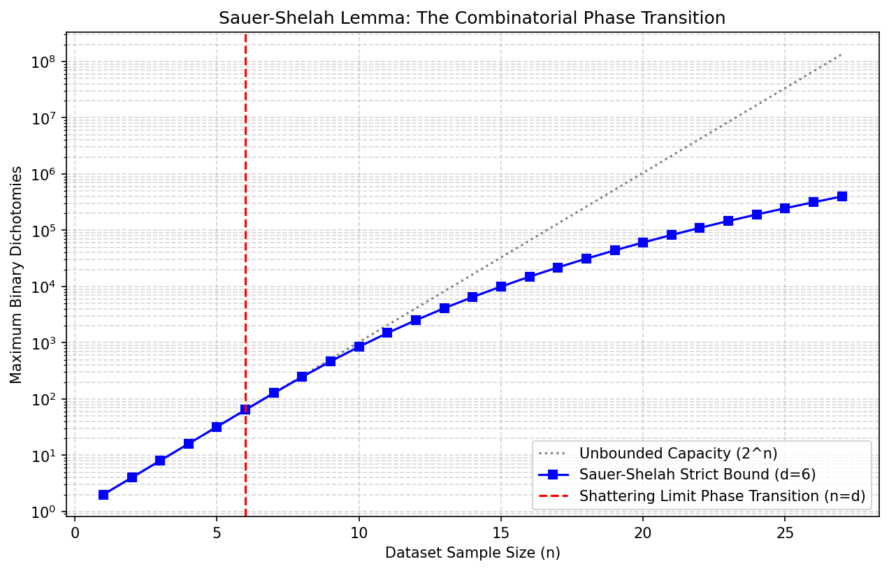
Demo 1: Visualizing the Sauer-Shelah Phase Transition
This Python script visually executes the Sauer-Shelah combinatorial bound, isolating the exact threshold where infinite complexity transitions dynamically into constrained polynomial growth.
import matplotlib
matplotlib.use('Agg')
import numpy as np
import matplotlib.pyplot as plt
import math

def calculate_sauer_shelah_bound(n, d):
    """Computes the exact Sauer-Shelah binomial sum bound."""
    if n < d:
        return 2**n # Exact shattering occurs
    return sum(math.comb(n, i) for i in range(d + 1))

sample_sizes = np.arange(1, 28)
vc_dimension = 6

true_unbounded = 2.0**sample_sizes
theoretical_bounds = [calculate_sauer_shelah_bound(n, vc_dimension) for n in sample_sizes]

plt.figure(figsize=(10, 6))
plt.semilogy(sample_sizes, true_unbounded, label='Unbounded Capacity (2^n)', linestyle=':', color='gray')
plt.semilogy(sample_sizes, theoretical_bounds, label=f'Sauer-Shelah Strict Bound (d={vc_dimension})', marker='s', color='blue')

# Demarcating the exact phase transition
plt.axvline(x=vc_dimension, color='red', linestyle='--', label='Shattering Limit Phase Transition (n=d)')

plt.xlabel('Dataset Sample Size (n)')
plt.ylabel('Maximum Binary Dichotomies')
plt.title('Sauer-Shelah Lemma: The Combinatorial Phase Transition')
plt.legend()
plt.grid(True, which='both', linestyle='--', alpha=0.5)
plt.savefig('figures/03-2-demo1.png', dpi=150, bbox_inches='tight')
plt.close()
Demo 2: Monte Carlo Simulation of \(L_1\) Rademacher Scaling
This demonstration computes the empirical Rademacher complexity of an \(L_1\)-bounded hypothesis class across exponentially expanding dimensions, validating the slow logarithmic scaling derived in our geometric proofs.
import matplotlib
matplotlib.use('Agg')
import numpy as np
import matplotlib.pyplot as plt

np.random.seed(42)
n_samples = 300      # Fixed Sample Count
weight_bound = 1.0   # Fixed L1 Norm Geometry
data_bound = 1.0     # Fixed L_infinity Input Space

dimensions = np.logspace(1, 5, 12).astype(int)
simulated_complexities = []

for d in dimensions:
    # Uniformly generated continuous data within L_inf bounds
    X = np.random.uniform(-data_bound, data_bound, size=(n_samples, d))

    mc_iterations = 40
    empirical_estimates = []

    for _ in range(mc_iterations):
        rad_signs = np.random.choice([-1, 1], size=(n_samples, 1))
        # Computation of the core Rademacher vector sum projection
        projected_sum = np.sum(rad_signs * X, axis=0) / n_samples
        # The supremum across the L1 simplex ball is cleanly the maximum absolute projection
        supremum_eval = weight_bound * np.max(np.abs(projected_sum))
        empirical_estimates.append(supremum_eval)

    simulated_complexities.append(np.mean(empirical_estimates))

plt.figure(figsize=(10, 6))
plt.plot(dimensions, simulated_complexities, marker='o', label='Simulated Rademacher Expectation', color='purple')

# Strict Mathematical Upper Bound evaluation
theoretical_asymptote = weight_bound * data_bound * np.sqrt(2 * np.log(2 * dimensions) / n_samples)
plt.plot(dimensions, theoretical_asymptote, linestyle='--', color='orange', label='Theoretical Asymptote O(sqrt(log(d)/n))')

plt.xscale('log')
plt.xlabel('Ambient Feature Dimension (d)')
plt.ylabel('Empirical Rademacher Complexity Magnitude')
plt.title('Validation of Logarithmic Scaling in L1-Regularized Metric Spaces')
plt.legend()
plt.grid(True, which='both', linestyle=':', alpha=0.8)
plt.savefig('figures/03-2-demo2.png', dpi=150, bbox_inches='tight')
plt.close()
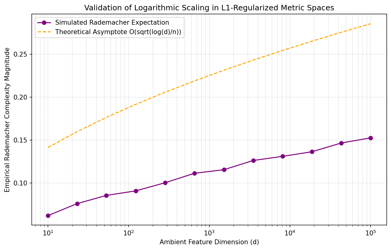
These rigorous programmatic models empirically reflect the absolute exactness of the mathematical complexities and bounding principles strictly established throughout the theoretical sections of this chapter.