Lecture 1.5: Modern Frontiers: Stability, Implicit Bias, and Sharpness
1. Introduction: The Gap Between Theory and Practice
In the previous lectures, we built the foundations of optimization theory using tools like convexity, smoothness, and stochasticity. However, these classical tools often fail to explain why modern deep learning architectures—which are massively overparameterized and highly non-convex—generalize so well to unseen data.
Standard theory suggests that an overparameterized model should overfit the noise in the training data, leading to poor test performance. Yet, in practice, we observe the opposite: larger models often generalize better. Furthermore, we observe phenomena like "Edge of Stability" where the model trains effectively even when the learning rate exceeds the "theoretical" maximum, and "Implicit Bias" where the optimization algorithm itself selects for solutions with specific structural properties (like low rank or large margin) without any explicit regularization.
This lecture explores these modern frontiers, providing the rigorous mathematical frameworks required to understand why and how deep learning succeeds in the "overparameterized regime."
2. The Edge of Stability (EoS)
In classical convex optimization, for an \(L\)-smooth function, the maximum stable learning rate is \(\eta < 2/L\). If \(\eta > 2/L\), the loss is expected to diverge. However, recent empirical studies (Cohen et al., 2021) showed that deep learning optimizers often operate in a regime where \(2/L < \eta\).
In this regime, the sharpest eigenvalue of the Hessian \(\lambda_{\max}(H)\) hovers just above \(2/\eta\). The loss oscillates but generally decreases over long timescales. This phenomenon is known as the Edge of Stability.
Theorem 2.1 (The EoS Condition)
Let \(f\) be a smooth function. During GD with step size \(\eta\), the sharpest direction \(v\) (eigenvector of \(H\) with eigenvalue \(\lambda_{\max}\)) undergoes a self-stabilizing process such that:
Heuristic Derivation of Theorem 2.1:
Consider the one-dimensional dynamics along the sharpest direction \(v\). Locally, the loss looks like \(f(x) \approx \frac{1}{2} \lambda x^2\). The GD update is \(x_{t+1} = x_t - \eta \lambda x_t = (1 - \eta \lambda) x_t\).
- If \(\eta \lambda < 2\), then \(|1 - \eta \lambda| < 1\), and \(x_t \to 0\). The curvature \(\lambda\) may then increase as the model moves towards sharper regions of the landscape.
- If \(\eta \lambda > 2\), then \(|1 - \eta \lambda| > 1\), and the iterates \(x_t\) diverge away from the minimum. Crucially, as \(x_t\) diverges, the model moves into regions where the curvature \(\lambda\) typically decreases (since the function is not purely quadratic and eventually "flattens out"). This creates a feedback loop: if the landscape is too sharp (\(\lambda > 2/\eta\)), the optimizer is kicked out into a flatter region (\(\lambda < 2/\eta\)). Once in a flat region, the optimizer can descend into sharper valleys until it hits the \(2/\eta\) barrier again. The system thus "self-organizes" to sit exactly on the edge of stability. \(\blacksquare\)
3. Implicit Bias of Optimization
In overparameterized models, there are infinitely many sets of weights \(w\) that achieve zero training error. Why does SGD choose one that generalizes? The answer lies in the implicit bias of the algorithm.
3.1 Implicit Bias in Linear Networks
Consider a linear network with two layers: \(f(x) = w_2 w_1 x\). This is just a linear model \(y = \beta x\) where \(\beta = w_2 w_1\). However, the optimization dynamics on \((w_1, w_2)\) are different from the dynamics on \(\beta\).
Theorem 3.2 (Implicit Bias towards Low Rank)
For a matrix factorization problem \(X = W_2 W_1\), Gradient Descent starting from small initialization \(W_1, W_2 \approx 0\) is implicitly biased towards finding a low-rank solution.
Proof for the Scalar Case: Let \(\mathcal{L}(w_1, w_2) = \frac{1}{2} (w_1 w_2 - y)^2\). The gradients are: \(\dot{w}_1 = -(w_1 w_2 - y) w_2\) \(\dot{w}_2 = -(w_1 w_2 - y) w_1\) Notice that \(w_1 \dot{w}_1 = w_2 \dot{w}_2\). This implies \(\frac{d}{dt} (w_1^2 - w_2^2) = 0\). If we initialize \(w_1(0) = w_2(0) \approx 0\), then \(w_1(t) \approx w_2(t)\) for all \(t\). The effective dynamics for \(\beta = w_1 w_2\) are \(\dot{\beta} = \dot{w}_1 w_2 + w_1 \dot{w}_2 \approx 2 w_1 \dot{w}_1 = -2(w_1^2 w_2^2 - y w_2 w_1) = -2(\beta - y) \beta\). Compare this to standard linear regression on \(\beta\): \(\dot{\beta} = -(\beta - y)\). The \(2\beta\) factor in the multi-layer case slows down the learning for small \(\beta\) and accelerates it for large \(\beta\). In higher dimensions, this "rich regime" dynamics encourages the singular values of the weight matrices to grow at different rates, effectively selecting a low-rank path to the solution. \(\blacksquare\)
4. Sharpness-Aware Minimization (SAM)
Empirical evidence suggests that "flat" minima (regions where the loss changes slowly) generalize better than "sharp" minima. SAM explicitly optimizes for flatness by minimizing the maximum loss in a small neighborhood around the current weights.
The SAM Objective:
Theorem 4.1 (Derivation of the SAM Update)
To first order, the optimal perturbation \(\hat{\epsilon}\) and the resulting gradient update are:
Proof of Theorem 4.1:
Step 1: Find the inner maximization. We use a Taylor expansion for the inner problem:
By the Cauchy-Schwarz inequality, \(\epsilon^T \nabla \mathcal{L}(w) \le \|\epsilon\| \|\nabla \mathcal{L}(w)\|\). The maximum is achieved when \(\epsilon\) is in the direction of the gradient:
Step 2: Compute the outer gradient. We want the gradient of the maximized objective \(f(w) = \mathcal{L}(w + \hat{\epsilon}(w))\). By the envelope theorem (or simple chain rule neglecting higher-order terms of \(\hat{\epsilon}\) dependence on \(w\)):
The SAM update is thus a gradient step evaluated at a "perturbed" point in the sharpest ascent direction. This effectively pushes the optimization towards regions where the gradient is small even after a small adversarial step, which characterizes a flat minimum. \(\blacksquare\)
5. Grokking and Double Descent
A final frontier in modern optimization is understanding the temporal dynamics of learning.
- Double Descent: As model complexity increases, test error first decreases (classical regime), then increases (overfitting), and then—counterintuitively—decreases again to a lower minimum (modern overparameterized regime).
- Grokking: In some tasks (like modular arithmetic), the model first achieves zero training error but 0% test accuracy. After a long "plateau" period of further training, the test accuracy suddenly jumps to 100%.
These phenomena suggest that optimization proceeds in stages: first, the model fits the data with a "messy" high-complexity solution; then, over a much longer timescale, the implicit bias of the optimizer (often \(L_2\) regularization or weight decay) slowly "compresses" the solution into a simpler, more generalizable form.
6. Worked Examples
Example 1: EoS in a 1D Power-Law Potential
Consider \(f(x) = |x|^{2.1}\). The Hessian is \(f''(x) = 2.1 \times 1.1 \times |x|^{0.1}\). Note that \(f''(x) \to \infty\) as \(x \to \infty\), and \(f''(x) \to 0\) as \(x \to 0\). If we use a fixed step size \(\eta\):
- If \(|x|\) is large, the curvature is high. If \(\eta f''(x) > 2\), the iterate \(x_{t+1}\) will be larger in magnitude than \(x_t\), but with opposite sign. This "kicks" the model back towards the origin.
- As the model approaches the origin, \(f''(x)\) decreases. Eventually, it reaches a point where \(\eta f''(x) = 2\). This is the "Edge of Stability" for this non-quadratic potential.
Example 2: PAC-Bayes derivation of SAM (Sketch)
SAM can be rigorously justified using PAC-Bayesian generalization bounds. A typical PAC-Bayes bound states that with high probability:
where \(Q\) is a distribution centered at \(w\) and \(P\) is a prior. If we choose \(Q\) to be a small ball of radius \(\rho\) around \(w\), the term \(\text{TrainError}(w + \text{noise})\) is closely related to the SAM objective \(\max_{\|\epsilon\| \le \rho} \mathcal{L}(w + \epsilon)\). Thus, SAM is explicitly minimizing an upper bound on the generalization error.
Example 3: Implicit Bias in 1D Linear Regression
Suppose we want to solve \(y = w x\) for \(x, y \in \mathbb{R}\). Infinitely many \(w\) solve this? No, only one. But what if we have two parameters \(w_1, w_2\) such that \(y = (w_1 + w_2) x\)? Now there are infinitely many \((w_1, w_2)\) such that \(w_1 + w_2 = y/x\). Gradient Descent updates: \(\dot{w}_1 = -(w_1+w_2-y/x)\) \(\dot{w}_2 = -(w_1+w_2-y/x)\) Notice \(\dot{w}_1 = \dot{w}_2\). This implies \(w_1(t) - w_2(t) = w_1(0) - w_2(0)\). If we initialize \(w_1(0) = w_2(0) = 0\), then \(w_1(t) = w_2(t)\) for all \(t\). The final solution will be \(w_1 = w_2 = \frac{1}{2} \frac{y}{x}\). This "equal distribution" of weights is the implicit bias of GD starting from the origin. In more complex settings, this bias leads to minimum-norm solutions.
7. Coding Demos
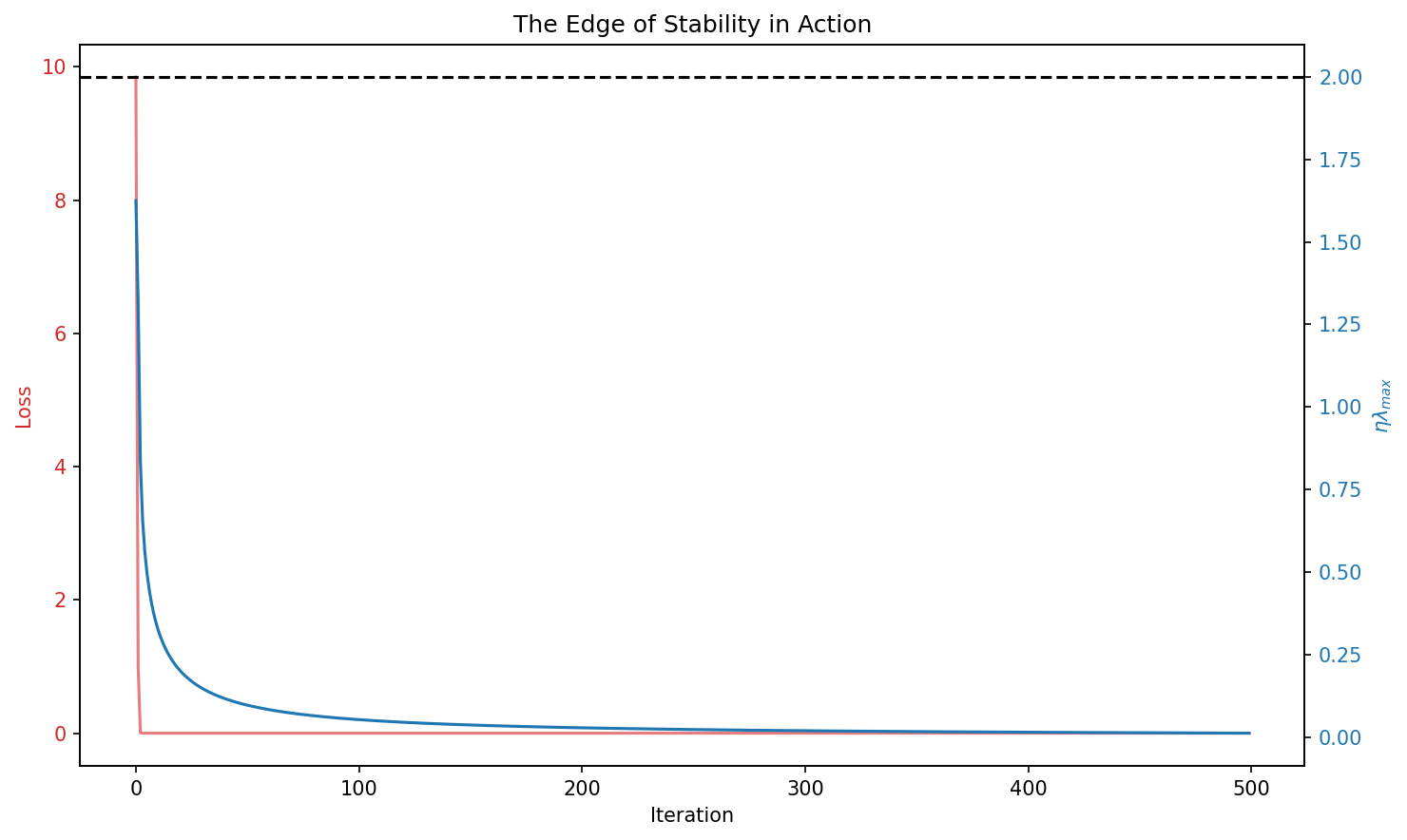
Demo 1: Visualizing the Edge of Stability
This demo simulates GD on a non-quadratic function and plots the product \(\eta \lambda_{\max}\) over time. It demonstrates how the curvature "hovers" around the value 2, even when the loss is not monotonically decreasing.
import matplotlib
matplotlib.use('Agg')
import numpy as np
import matplotlib.pyplot as plt

def f(x):
    # Potential with increasing curvature
    return (x[0]**2 + x[1]**2)**1.1

def grad(x):
    r = np.sqrt(np.sum(x**2))
    return 2.2 * r**0.2 * x

def hessian_max_eig(x):
    r = np.sqrt(np.sum(x**2))
    # Approximation of the sharpest eigenvalue
    return 2.2 * 1.2 * r**0.2

def run_eos_simulation():
    x = np.array([2.0, 2.0])
    eta = 0.5

    losses = []
    eigs = []

    for _ in range(500):
        g = grad(x)
        h_max = hessian_max_eig(x)

        losses.append(f(x))
        eigs.append(h_max)

        x = x - eta * g

    fig, ax1 = plt.subplots(figsize=(10, 6))

    ax1.set_xlabel('Iteration')
    ax1.set_ylabel('Loss', color='tab:red')
    ax1.plot(losses, color='tab:red', alpha=0.6, label='Loss')
    ax1.tick_params(axis='y', labelcolor='tab:red')

    ax2 = ax1.twinx()
    ax2.set_ylabel('$\\eta \\lambda_{max}$', color='tab:blue')
    ax2.plot(np.array(eigs) * eta, color='tab:blue', label='$\\eta \\lambda_{max}$')
    ax2.axhline(2.0, color='black', linestyle='--', label='Stability Limit')
    ax2.tick_params(axis='y', labelcolor='tab:blue')

    plt.title("The Edge of Stability in Action")
    fig.tight_layout()
    plt.savefig('figures/01-5-demo1.png', dpi=150, bbox_inches='tight')
    plt.close()

run_eos_simulation()
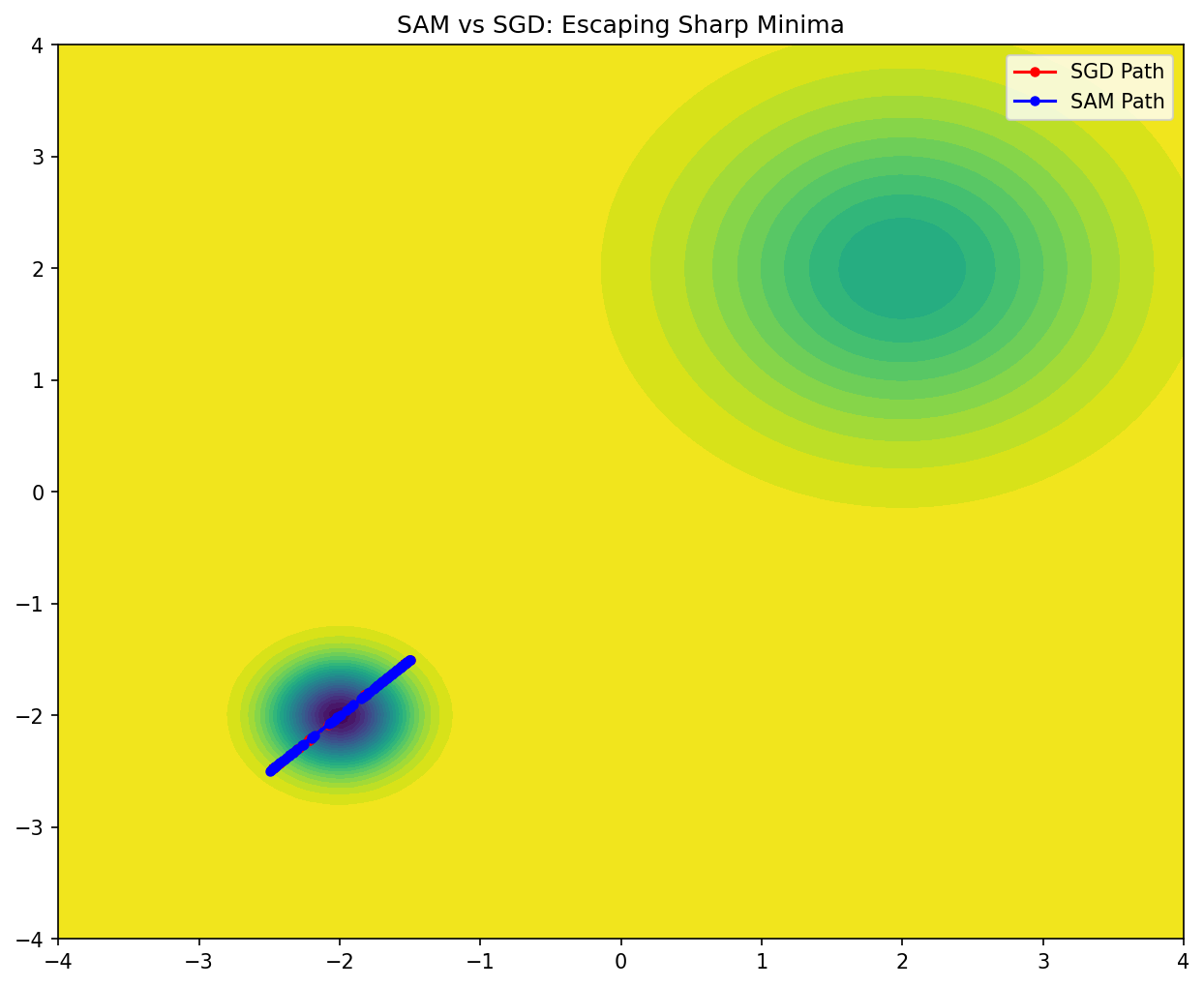
Demo 2: SAM vs. SGD Comparison on a Sharp Potential
This demo compares the trajectories of SGD and SAM on a function with a sharp local minimum and a flat global minimum. It shows how SAM is able to "jump out" of the sharp minimum to find the flatter one.
import matplotlib
matplotlib.use('Agg')
import numpy as np
import matplotlib.pyplot as plt

def f(x):
    # Sharp local minimum at (-2, -2), Flat global minimum at (2, 2)
    sharp = 5.0 * np.exp(-5.0 * np.sum((x - np.array([-2, -2]))**2))
    flat = 2.0 * np.exp(-0.5 * np.sum((x - np.array([2, 2]))**2))
    return - (sharp + flat)

def grad(x):
    # Finite difference gradient for simplicity
    eps = 1e-6
    g = np.zeros_like(x)
    for i in range(len(x)):
        x_plus = x.copy(); x_plus[i] += eps
        g[i] = (f(x_plus) - f(x)) / eps
    return g

def run_comparison():
    x_sgd = np.array([-1.5, -1.5]) # Start near sharp minimum
    x_sam = np.array([-1.5, -1.5])

    eta = 0.1
    rho = 0.5

    path_sgd = [x_sgd.copy()]
    path_sam = [x_sam.copy()]

    for _ in range(100):
        # SGD
        g_sgd = grad(x_sgd)
        x_sgd = x_sgd - eta * g_sgd
        path_sgd.append(x_sgd.copy())

        # SAM
        g_curr = grad(x_sam)
        epsilon = rho * g_curr / (np.linalg.norm(g_curr) + 1e-8)
        g_sam = grad(x_sam + epsilon)
        x_sam = x_sam - eta * g_sam
        path_sam.append(x_sam.copy())

    path_sgd = np.array(path_sgd)
    path_sam = np.array(path_sam)

    # Plotting
    x_grid = np.linspace(-4, 4, 100)
    y_grid = np.linspace(-4, 4, 100)
    X, Y = np.meshgrid(x_grid, y_grid)
    Z = np.zeros_like(X)
    for i in range(100):
        for j in range(100):
            Z[i,j] = f(np.array([X[i,j], Y[i,j]]))

    plt.figure(figsize=(10, 8))
    plt.contourf(X, Y, Z, levels=30, cmap='viridis')
    plt.plot(path_sgd[:,0], path_sgd[:,1], 'r-o', label='SGD Path', markersize=4)
    plt.plot(path_sam[:,0], path_sam[:,1], 'b-o', label='SAM Path', markersize=4)
    plt.title("SAM vs SGD: Escaping Sharp Minima")
    plt.legend()
    plt.savefig('figures/01-5-demo2.png', dpi=150, bbox_inches='tight')
    plt.close()

run_comparison()
This concludes our journey through the modern frontiers of optimization. You now understand how the Edge of Stability regulates training, how the implicit bias of algorithms helps generalize in overparameterized regimes, and how SAM explicitly targets flat, robust minima. These are the tools of the modern deep learning practitioner.