9.5 Kernel Mean Embeddings and Maximum Mean Discrepancy (MMD)
Introduction
So far, we have used kernels to map individual data points into a Hilbert space: \(x \mapsto \phi(x)\). But what if we want to map an entire probability distribution into the RKHS?
This is the goal of Kernel Mean Embeddings. By representing distributions as points in an RKHS, we can use Hilbert space operations (like distance and inner products) to compare distributions, leading to the Maximum Mean Discrepancy (MMD). MMD is a cornerstone of modern two-sample testing, generative modeling (like MMD-GANs), and domain adaptation.
Kernel Mean Embeddings
Let \(\mathbb{P}\) be a probability distribution over \(\mathcal{X}\). Let \(\mathcal{H}\) be an RKHS with kernel \(k\).
Definition
The kernel mean embedding of \(\mathbb{P}\), denoted \(\mu_\mathbb{P} \in \mathcal{H}\), is defined as the expected feature map:
For this integral to be well-defined in \(\mathcal{H}\) (in the sense of a Bochner integral), we require \(\mathbb{E}_{X \sim \mathbb{P}} [\sqrt{k(X,X)}] < \infty\). If the kernel is bounded (e.g., Gaussian RBF \(k(x,x)=1\)), this holds for all probability distributions.
By the Riesz representation theorem and linearity of expectation, the inner product of any function \(f \in \mathcal{H}\) with the mean embedding yields the expected value of the function under the distribution:
Characteristic Kernels
An embedding is only useful if it is injective. If two different distributions map to the same point in the RKHS (\(\mu_\mathbb{P} = \mu_\mathbb{Q}\) but \(\mathbb{P} \neq \mathbb{Q}\)), we lose information.
Definition
A kernel \(k\) is characteristic if the mean embedding map \(\mathbb{P} \mapsto \mu_\mathbb{P}\) is injective. That is:
Theorem (Characteristic kernels and Bochner)
A translation-invariant kernel \(k(x, y) = k(x-y)\) on \(\mathbb{R}^d\) is characteristic if and only if the support of its Fourier transform (from Bochner's Theorem) is the entire \(\mathbb{R}^d\).
Proof Outline: 1. Assume \(\mu_\mathbb{P} = \mu_\mathbb{Q}\). This means \(\langle f, \mu_\mathbb{P} \rangle = \langle f, \mu_\mathbb{Q} \rangle\) for all \(f \in \mathcal{H}\). 2. Thus, \(\mathbb{E}_\mathbb{P}[f(X)] = \mathbb{E}_\mathbb{Q}[f(X)]\) for all \(f \in \mathcal{H}\). 3. For translation-invariant kernels, Bochner's theorem implies \(\mathcal{H}\) is closely related to Fourier transforms. 4. If the kernel's Fourier spectrum covers all of \(\mathbb{R}^d\) (like the Gaussian kernel), the RKHS is dense in the space of continuous functions vanishing at infinity \(C_0(\mathbb{R}^d)\). 5. By the Riesz-Markov-Kakutani representation theorem, if expectations of all \(C_0\) functions match, the probability measures must be strictly identical (\(\mathbb{P} = \mathbb{Q}\)). 6. If the Fourier transform has zero support on some frequency band, we can construct two distributions whose characteristic functions differ only in that band, causing a collision in the mean embedding. \(\blacksquare\)
Consequence: The Gaussian RBF kernel and Laplacian kernel are characteristic. The linear kernel \(k(x,y)=x^Ty\) is not characteristic (its embedding is just the first moment/mean of the distribution; distributions with the same mean will collide).
Maximum Mean Discrepancy (MMD)
We can now define a distance between two probability distributions \(\mathbb{P}\) and \(\mathbb{Q}\) simply as the RKHS distance between their embeddings.
Definition (MMD)
If \(k\) is a characteristic kernel, \(\text{MMD}(\mathbb{P}, \mathbb{Q}) = 0 \iff \mathbb{P} = \mathbb{Q}\). Thus, MMD is a valid metric on probability distributions.
Integral Probability Metric View
MMD can be equivalently written as a variational problem. Using the definition of the dual norm:
This is the Integral Probability Metric (IPM) formulation. MMD finds the smooth function \(f\) (the "critic") in the unit ball of the RKHS that maximally distinguishes the two distributions.
Explicit Empirical Estimator
Expanding the squared MMD norm yields a form that depends only on kernel evaluations:
Given finite samples \(X = \{x_1, \dots, x_n\} \sim \mathbb{P}\) and \(Y = \{y_1, \dots, y_m\} \sim \mathbb{Q}\), we construct the unbiased empirical estimator (removing the diagonal terms where \(x_i = x_i\)):
This estimator runs in \(O((n+m)^2)\) time.
MMD Asymptotics and Two-Sample Testing
A primary use of MMD is the Two-Sample Test: deciding whether two sets of samples \(X\) and \(Y\) come from the same distribution (\(H_0: \mathbb{P} = \mathbb{Q}\)) or different distributions (\(H_1: \mathbb{P} \neq \mathbb{Q}\)).
To set a rejection threshold, we need the asymptotic distribution of \(\widehat{\text{MMD}^2}_u\) under the null hypothesis.
Theorem (Asymptotics of MMD)
Assume \(m=n\) for simplicity. 1. Under \(H_1 (\mathbb{P} \neq \mathbb{Q})\): \(\widehat{\text{MMD}^2}_u\) is asymptotically normal.
- Under \(H_0 (\mathbb{P} = \mathbb{Q})\): \(\widehat{\text{MMD}^2}_u\) is a degenerate U-statistic. Its asymptotic distribution is an infinite mixture of Chi-squared variables.
where \(\mathcal{Z}_l \sim \mathcal{N}(0,1)\) i.i.d., and \(\lambda_l\) are the eigenvalues of the integral operator \(\int \tilde{k}(x, y) \psi_l(y) d\mathbb{P}(y) = \lambda_l \psi_l(x)\), with the centered kernel \(\tilde{k}(x, y) = k(x,y) - \mathbb{E}_x[k(x,y)] - \mathbb{E}_y[k(x,y)] + \mathbb{E}_{x,y}[k(x,y)]\).
Proof outline of \(H_0\) Asymptotics: Since \(\mathbb{P} = \mathbb{Q}\), the first order term of the U-statistic Hoeffding decomposition vanishes (hence "degenerate"). The limiting distribution of a degenerate U-statistic of order 2 is characterized by the spectral decomposition of its kernel. Applying Mercer's Theorem to the centered kernel \(\tilde{k}\) gives \(\tilde{k}(x,y) = \sum \lambda_l \psi_l(x) \psi_l(y)\). Substituting this into the U-statistic and applying the Central Limit Theorem to the empirical averages of \(\psi_l(x)\) yields the infinite sum of independent \(\chi^2_1\) variables. \(\blacksquare\)
Because the null distribution involves unknown eigenvalues \(\lambda_l\) (which depend on the unknown \(\mathbb{P}\)), we typically compute the p-value via permutation testing.
Worked Examples
Example 1: The Witness Function
The function \(f\) that maximizes the discrepancy in the IPM view is called the witness function. By taking the Fréchet derivative of the dual norm formulation, it can be shown that the optimal witness function (up to scaling) is exactly the difference of the mean embeddings:
Where this function is positive, \(\mathbb{P}\) has higher density than \(\mathbb{Q}\). Where it is negative, \(\mathbb{Q}\) has higher density.
Example 2: Mean Embedding with Linear Kernel
If \(k(x,y) = x^T y\), then \(\mu_\mathbb{P} = \mathbb{E}[X] \in \mathbb{R}^d\). \(\text{MMD}^2(\mathbb{P}, \mathbb{Q}) = \|\mathbb{E}[X] - \mathbb{E}[Y]\|_2^2\). This only tests for differences in the means of the distributions, ignoring variance, skewness, etc., which proves why the linear kernel is not characteristic.
Example 3: Training Generative Models (MMD-GAN)
Generative Adversarial Networks usually use a neural network discriminator. MMD-GAN replaces the discriminator with MMD. Let \(Y \sim \mathbb{Q}\) be real data, and \(X = G_\theta(Z)\) be generated data. We train the generator to minimize the MMD between \(G_\theta(Z)\) and \(Y\) using gradients backpropagated through the MMD estimator.
Coding Demos
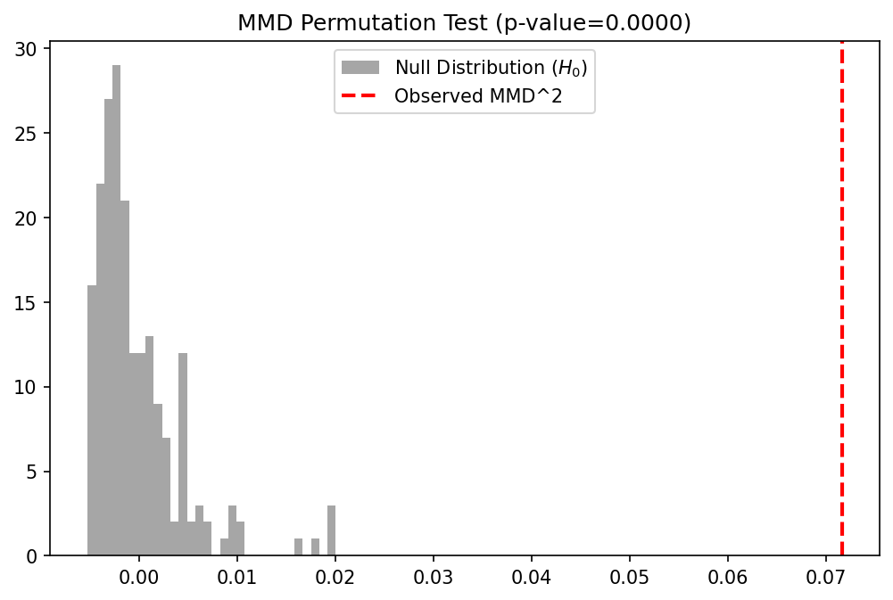
Demo 1: MMD Two-Sample Test with Permutations
We implement the unbiased MMD estimator and use a permutation test to calculate the p-value for testing if two datasets are from the same distribution.
import matplotlib
matplotlib.use('Agg')
import numpy as np
import matplotlib.pyplot as plt
from sklearn.metrics.pairwise import rbf_kernel

def mmd_squared_unbiased(K_XX, K_YY, K_XY):
    n = K_XX.shape[0]
    m = K_YY.shape[0]

    # Remove diagonals
    np.fill_diagonal(K_XX, 0)
    np.fill_diagonal(K_YY, 0)

    term_XX = np.sum(K_XX) / (n * (n - 1))
    term_YY = np.sum(K_YY) / (m * (m - 1))
    term_XY = np.sum(K_XY) / (n * m)

    return term_XX + term_YY - 2 * term_XY

def compute_mmd(X, Y, gamma=1.0):
    K_XX = rbf_kernel(X, X, gamma=gamma)
    K_YY = rbf_kernel(Y, Y, gamma=gamma)
    K_XY = rbf_kernel(X, Y, gamma=gamma)
    return mmd_squared_unbiased(K_XX, K_YY, K_XY)

# Generate data
np.random.seed(42)
# P is N(0, 1), Q is N(0.5, 1) - slight shift
n_samples = 200
X = np.random.normal(0, 1, size=(n_samples, 1))
Y = np.random.normal(0.5, 1, size=(n_samples, 1))

# 1. Compute actual MMD
gamma_val = 1.0
actual_mmd = compute_mmd(X, Y, gamma=gamma_val)
print(f"Observed MMD^2: {actual_mmd:.5f}")

# 2. Permutation Test for p-value
n_permutations = 200
pooled_data = np.vstack([X, Y])
total_samples = 2 * n_samples

mmd_null = np.zeros(n_permutations)
for i in range(n_permutations):
    perm_idx = np.random.permutation(total_samples)
    pooled_perm = pooled_data[perm_idx]
    X_perm = pooled_perm[:n_samples]
    Y_perm = pooled_perm[n_samples:]
    mmd_null[i] = compute_mmd(X_perm, Y_perm, gamma=gamma_val)

p_value = np.mean(mmd_null >= actual_mmd)
print(f"P-value: {p_value:.4f}")

# 3. Plot Null Distribution
plt.figure(figsize=(8, 5))
plt.hist(mmd_null, bins=30, alpha=0.7, color='gray', label='Null Distribution ($H_0$)')
plt.axvline(actual_mmd, color='red', linestyle='dashed', linewidth=2, label='Observed MMD^2')
plt.title(f"MMD Permutation Test (p-value={p_value:.4f})")
plt.legend()
plt.savefig('figures/09-5-demo1.png', dpi=150, bbox_inches='tight')
plt.close()
Demo 2: Visualizing the Witness Function
We plot the witness function, showing where the RKHS has detected the difference between the distributions.
import matplotlib
matplotlib.use('Agg')
import numpy as np
import matplotlib.pyplot as plt
from sklearn.metrics.pairwise import rbf_kernel

# Reusing X, Y from previous demo
np.random.seed(42)
n_samples = 200
X = np.random.normal(0, 1, size=(n_samples, 1))
Y = np.random.normal(0.5, 1, size=(n_samples, 1))
gamma_val = 1.0

X_grid = np.linspace(-3, 4, 300).reshape(-1, 1)

# Compute E[k(x, X)] and E[k(x, Y)]
K_grid_X = rbf_kernel(X_grid, X, gamma=gamma_val)
K_grid_Y = rbf_kernel(X_grid, Y, gamma=gamma_val)

mu_P_grid = np.mean(K_grid_X, axis=1)
mu_Q_grid = np.mean(K_grid_Y, axis=1)

witness_function = mu_P_grid - mu_Q_grid

plt.figure(figsize=(10, 5))
plt.hist(X, bins=30, density=True, alpha=0.5, color='blue', label='Distribution P (X)')
plt.hist(Y, bins=30, density=True, alpha=0.5, color='orange', label='Distribution Q (Y)')
plt.plot(X_grid, witness_function, 'k-', linewidth=2, label='Witness Function $f_{witness}(x)$')
plt.axhline(0, color='gray', linestyle='--')
plt.title("Distributions and their RKHS Witness Function")
plt.legend()
plt.savefig('figures/09-5-demo2.png', dpi=150, bbox_inches='tight')
plt.close()
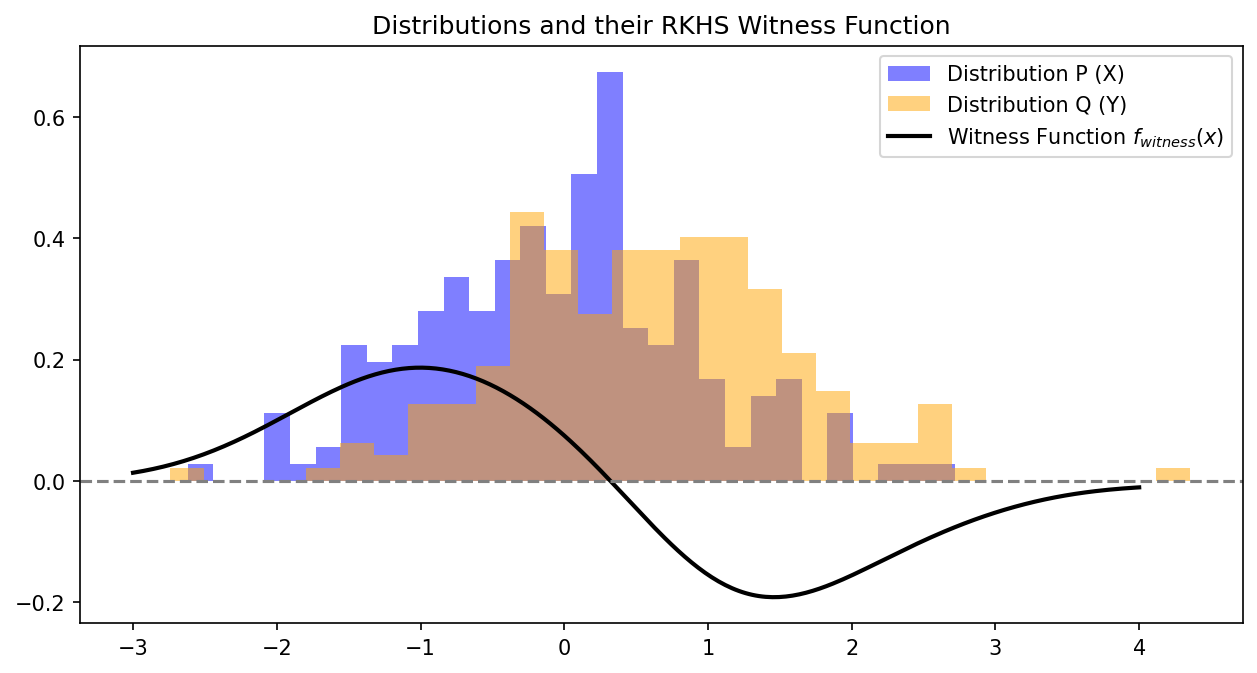 Observation: The witness function is positive where \(\mathbb{P}\) (blue) has more mass, and negative where \(\mathbb{Q}\) (orange) has more mass. It cleanly separates the discrepancy between the two geometries, acting as the optimal discriminator in the RKHS.