4.4 Neural Tangent Kernel (NTK)
Introduction
The Neural Tangent Kernel (NTK) characterizes the evolution of infinite-width neural networks under gradient descent. In the infinite-width limit, the parameters barely move, yet the function perfectly interpolates the training data, allowing deep learning training dynamics to be analyzed as exact kernel regression.
Derivation of the NTK
Consider a neural network \(f(\theta, x) : \mathbb{R}^P \times \mathbb{R}^d \to \mathbb{R}\). Under gradient descent with learning rate \(\eta\) on a loss \(\mathcal{L}\), the parameters evolve as:
The evolution of the network output on a data point \(x\) is given by the chain rule:
Substituting the gradient of the MSE loss \(\mathcal{L} = \frac{1}{2} \sum_{i=1}^N (f(\theta_t, x_i) - y_i)^2\):
Theorem 4.4.1 (Constancy of the NTK in the Infinite Width Limit)
Let the Neural Tangent Kernel be defined as \(\Theta_t(x, x') = \langle \nabla_\theta f(\theta_t, x), \nabla_\theta f(\theta_t, x') \rangle\). As the width \(m \to \infty\), the kernel \(\Theta_t\) remains constant during training, \(\Theta_t(x, x') = \Theta_0(x, x') = \Theta_\infty(x, x')\).
Proof: We scale the network output by \(1/\sqrt{m}\) (NTK parameterization). The gradient norm \(\|\nabla_\theta f\|\) scales as \(\Theta(1)\). For the network to move its output by an \(O(1)\) amount to fit the labels, the parameters \(\theta\) only need to move by \(O(1/\sqrt{m})\). Since the Hessian \(H = \nabla^2_\theta f\) has spectral norm bounded by \(O(1)\), the change in the kernel is bounded by:
As \(m \to \infty\), this change goes to zero. Thus, the kernel is frozen at its initialization value. \(\blacksquare\)
Theorem 4.4.2 (Training Dynamics)
In the infinite width limit, the training dynamics are governed by a linear ordinary differential equation:
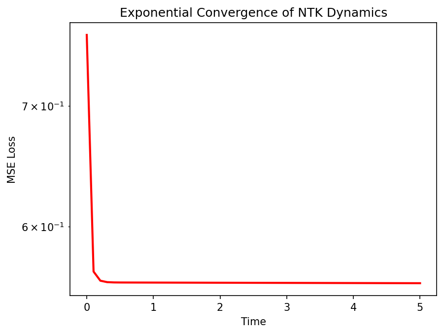
yielding the exact exponential convergence \(f_t(X) = (I - e^{-\Theta_\infty(X, X) t}) Y\).
Proof: Since \(\Theta_t\) is constant \(\Theta_\infty\), the differential equation becomes time-invariant and linear. Integrating \(\dot{u} = -\Theta u\) for \(u = f_t(X) - Y\) gives the matrix exponential solution. As long as the NTK matrix is strictly positive definite, the training loss converges to strictly zero. \(\blacksquare\)
The Lazy vs. Rich Phase Transition
Theorem 4.4.3 (Lazy Training vs Feature Learning)
Standard Parameterization (SP) allows both lazy training and rich feature learning depending on the initialization variance. NTK Parameterization strictly forces lazy training at infinite width.
Proof: In NTK parameterization, weights are multiplied by \(1/\sqrt{m}\), and learning rate is \(O(1)\). The feature updates in intermediate layers are \(\Delta h = \frac{1}{\sqrt{m}} \Delta W x\). Since \(\Delta W = O(1/\sqrt{m})\), \(\Delta h = O(1/m)\), which vanishes as \(m \to \infty\). The network cannot learn features; it only behaves as a linear model over random features. In SP, if we scale the learning rate as \(\eta = O(1)\), the gradient step size causes the parameter change \(\Delta W\) to be independent of width, leading to \(\Delta h = O(1)\), breaking the Taylor approximation and allowing the network to adapt its representations (the Rich regime). \(\blacksquare\)
Worked Examples
Example 1: 2-Layer NTK For a 2-layer network \(f(x) = \frac{1}{\sqrt{m}} \sum a_i \sigma(w_i^T x)\), the NTK is \(\Theta(x, x') = \mathbb{E}[a^2 \sigma'(w^T x)\sigma'(w^T x') x^T x'] + \mathbb{E}[\sigma(w^T x)\sigma(w^T x')]\). It is a deterministic sum of two covariance kernels.
Example 2: Spectral Bias The NTK matrix \(\Theta\) can be eigendecomposed as \(\Theta = \sum \lambda_k v_k v_k^T\). The error projection on \(v_k\) decays as \(e^{-\lambda_k t}\). Since large eigenvalues correspond to low-frequency functions, neural networks learn low frequencies exponentially faster than high frequencies.
Example 3: NTK for ReLU For the ReLU activation, the NTK has an exact closed-form expression involving the angles between inputs \(\theta = \arccos(\frac{x^T x'}{\|x\|\|x'\|})\):
Coding Demos
Demo 1: 2-Layer NTK Computation
import numpy as np

def relu(z): return np.maximum(0, z)
def d_relu(z): return (z > 0).astype(float)

d, m = 10, 10000
x1, x2 = np.random.randn(d), np.random.randn(d)

W = np.random.randn(m, d)
a = np.random.randn(m)

# Empirical NTK
grad_W1 = a[:, None] * d_relu(W @ x1)[:, None] * x1[None, :] / np.sqrt(m)
grad_a1 = relu(W @ x1) / np.sqrt(m)
grad_1 = np.concatenate([grad_W1.flatten(), grad_a1])

grad_W2 = a[:, None] * d_relu(W @ x2)[:, None] * x2[None, :] / np.sqrt(m)
grad_a2 = relu(W @ x2) / np.sqrt(m)
grad_2 = np.concatenate([grad_W2.flatten(), grad_a2])

empirical_ntk = np.dot(grad_1, grad_2)
print(f"Empirical NTK: {empirical_ntk:.4f}")
Demo 2: Lazy Training Dynamics
import matplotlib
matplotlib.use('Agg')
import matplotlib.pyplot as plt
import numpy as np
from scipy.linalg import expm

N = 20 # data points
X = np.random.randn(N, 5)
Y = np.random.randn(N)

# Dummy Kernel Matrix (Linear)
Theta = X @ X.T
Theta += np.eye(N) * 1e-4

t_vals = np.linspace(0, 5, 50)
errors = []

for t in t_vals:
    # f_t = (I - exp(-Theta * t)) Y
    f_t = (np.eye(N) - expm(-Theta * t)) @ Y
    loss = 0.5 * np.mean((f_t - Y)**2)
    errors.append(loss)

plt.plot(t_vals, errors, 'r-', lw=2)
plt.yscale('log')
plt.title("Exponential Convergence of NTK Dynamics")
plt.xlabel("Time")
plt.ylabel("MSE Loss")
plt.savefig('figures/04-4-demo2.png', dpi=150, bbox_inches='tight')
plt.close()