Chapter 2.2: Depth Efficiency and Separation Theorems: The Hierarchical Advantage
1. Introduction: The Failure of Flat Representations
The Universal Approximation Theorem (UAT) established the foundational possibility that a single hidden layer could, in principle, represent any continuous function. However, this theoretical existence proof masks a profound practical limitation: the "Curse of Dimensionality." For many natural functions, the number of neurons required in a shallow network scales exponentially with the input dimension \(d\), making them physically impossible to realize.
The empirical revolution of deep learning, which began in the mid-2000s, was built on the heuristic that stacking layers allows for hierarchical feature extraction. But is this stacking mathematically necessary? In 2016, a series of breakthrough papers provided rigorous Depth Separation Theorems, proving that there are functional classes that can be efficiently approximated by deep networks but require exponentially large shallow networks.
This chapter provides a completely exhaustive, rigorous, and step-by-step mathematical treatment of these theorems. We will prove Telgarsky's Sawtooth separation in 1D, Eldan and Shamir's radial separation in high dimensions, and establish the VC-dimension bounds that quantify the information-theoretic power of depth.
2. Mathematical Preliminaries: Piecewise Linear Complexity
Most modern deep networks utilize the Rectified Linear Unit (ReLU) activation function, \(\sigma(z) = \max(0, z)\). A ReLU network \(N: \mathbb{R}^d \to \mathbb{R}\) computes a function that is continuous and piecewise linear (CPW).
2.1 Quantifying Functional Complexity
To compare shallow and deep networks, we need a rigorous metric for "complexity." For CPW functions, this is the number of linear regions.
Definition 2.1.1 (Number of Segments)
For a function \(f: \mathbb{R} \to \mathbb{R}\), let \(S(f)\) be the number of linear segments in its graph.
Theorem 2.1.2 (Shallow Limit)
A neural network with a single hidden layer of \(m\) ReLU neurons computes a CPW function with at most \(m+1\) linear segments.
Proof:
- A single neuron \(\sigma(wx + b)\) has a single "kink" at \(x = -b/w\). To the left of this point, the function is constant (0); to the right, it is a line (\(wx+b\)).
- A shallow network is a linear combination of \(m\) such functions: \(N(x) = \sum_{j=1}^m v_j \sigma(w_j x + b_j) + c\).
- The points of non-differentiability of \(N(x)\) are restricted to the set of \(m\) kink points.
- \(m\) points on the real line can define at most \(m+1\) contiguous intervals.
- On each interval, the state of every ReLU (active or inactive) is fixed. The sum of linear functions is linear.
- Thus, \(N(x)\) has at most \(m+1\) affine segments. \(\blacksquare\)
2.2 The Multiplicative Power of Composition
The fundamental operation of a deep network is function composition: \(f(g(x))\).
Theorem 2.1.3 (Compositional Complexity)
If \(f\) and \(g\) are CPW functions with \(S_f\) and \(S_g\) segments respectively, then the composition \(h = f \circ g\) has at most \(S_f \cdot S_g\) segments.
Proof:
- Let the segments of \(g\) be \(J_1, \dots, J_{S_g}\). On each \(J_k\), \(g(x)\) is linear.
- The image \(g(J_k)\) is an interval in the domain of \(f\).
- As \(x\) traverses \(J_k\), \(g(x)\) can sweep across all \(S_f\) segments of \(f\).
- Each time \(g(x)\) enters a new segment of \(f\), the slope of \(f(g(x))\) can change.
- Thus, each of the \(S_g\) segments of \(g\) can be split into at most \(S_f\) sub-segments in the composition.
- Total segments \(\le S_f \cdot S_g\). \(\blacksquare\)
Crucial Insight: Addition adds segments (\(m+m=2m\)), but composition multiplies them (\(m \cdot m = m^2\)). This is the mathematical engine behind depth efficiency.
3. Telgarsky's Sawtooth Theorem: Exponential 1D Separation
In 2016, Matus Telgarsky proved that deep networks can create an exponential number of oscillations using only a linear number of parameters.
3.1 Constructing the Iterated Sawtooth
Definition 3.1.1 (The Base Sawtooth)
Define \(g: [0, 1] \to [0, 1]\) as:
This can be implemented by a 2-layer ReLU network with 3 hidden units: \(g(x) = \sigma(2x) - 2\sigma(2x - 1) + \sigma(2x - 2)\).
Definition 3.1.2 (The Iterated Map)
We define \(f_L(x)\) as the \(L\)-th iteration of \(g\):
3.2 Complexity of the Deep Sawtooth
Theorem 3.2.1 (The Exponential Explosion)
\(f_L(x)\) has exactly \(2^L\) linear segments.
Proof by Induction:
- Base Case (\(L=1\)): \(f_1 = g\) has 2 segments.
- Inductive Step: Assume \(f_{L-1}\) has \(2^{L-1}\) segments, each mapping a sub-interval \([a, b]\) bijectively to \([0, 1]\).
- Applying \(g\) to the output of \(f_{L-1}\) splits each of these \(2^{L-1}\) intervals into 2 new segments (one where \(g\) goes up, one where \(g\) goes down).
- Total segments in \(f_L = 2 \cdot 2^{L-1} = 2^L\). \(\blacksquare\)
3.3 The Separation Result
Theorem 3.3.1 (Telgarsky's Theorem)
For any \(L \in \mathbb{N}\), there exists a function \(f_L\) computable by a ReLU network of depth \(2L\) and width 3 such that any shallow network with \(m \le 2^{L-2}\) neurons satisfies:
Proof Sketch:
- \(f_L\) has \(2^L\) "teeth."
- \(S(x)\) has at most \(2^{L-2}+1\) segments.
- On most intervals where \(f_L\) oscillates, \(S(x)\) is purely linear and cannot track the oscillation.
- The error in approximating a triangle with a line is a constant fraction of the triangle's area.
- Summing over the domain yields the global \(L_1\) lower bound. \(\blacksquare\)
4. Multidimensional Separation: The Eldan-Shamir Theorem
Telgarsky's proof relies on oscillations. Eldan and Shamir (2016) proved a separation for a much simpler "bump" function in high dimensions.
4.1 The Curse of Ridge Functions
A shallow 2-layer network in \(\mathbb{R}^d\) computes: \(N(x) = \sum a_i \sigma(w_i^T x + b_i)\). Each term is a ridge function, which is constant in \(d-1\) directions. To approximate a radial "ball" or a localized bump, a shallow network must use an enormous number of ridge functions to "mask out" the infinite extent of each ridge.
Theorem 4.1.1 (Eldan-Shamir)
There exists a radial function \(f(x) = \phi(\|x\|)\) in \(\mathbb{R}^d\) that can be approximated to error \(\epsilon\) by a 3-layer network with \(\operatorname{poly}(d)\) neurons, but requires \(\exp(d)\) neurons for any 2-layer network.
5. Information-Theoretic Capacity: VC-Dimension and Bit Extraction
Another way to see the power of depth is through the Vapnik-Chervonenkis (VC) dimension.
Theorem 5.1.1 (Bartlett et al, 2019)
For a ReLU network with \(W\) parameters and \(L\) layers, the VC-dimension satisfies:
The Bit-Extraction Argument: Deep networks can perform "bit-extraction." Imagine a weight \(w = 0.b_1 b_2 b_3 \dots b_L\) (binary).
- A ReLU network can compute \(x \mapsto 2x - \lfloor 2x \rfloor\) to "shift" the bits.
- By stacking \(L\) layers, the network can extract the \(L\)-th bit of its own weight.
- This allows a deep network to "memorize" labels very efficiently, whereas a shallow network would have to store each bit in a separate parallel neuron. \(\blacksquare\)
6. Worked Examples
Example 6.1: Counting Linear Regions for \(f_3(x)\)
Target: \(f_3(x) = g(g(g(x)))\).
- \(g\) has 2 segments.
- \(f_3\) has \(2 \cdot 2 \cdot 2 = 8\) segments.
- A shallow network needs \(m \ge 8-1 = 7\) neurons.
-
A deep network uses 3 neurons per layer \(\times\) 3 layers = 9 neurons. Wait! For \(L=3\), the numbers are close. But for \(L=20\):
-
Shallow needs \(m \approx 2^{20} \approx 1,000,000\) neurons.
- Deep needs \(3 \times 20 = 60\) neurons. This is the exponential advantage.
Example 6.2: Approximating a Sphere in \(d=100\)
To approximate a sphere in 100D with error \(\epsilon\):
- 2-layer needs \(\approx (1/\epsilon)^{100}\) directions.
- 3-layer can compute \(x_1^2 + \dots + x_{100}^2\) using 100 parallel square-approximators. Each square takes \(\sim 20\) neurons. Total \(\sim 2000\) neurons. Deep networks are physically possible where shallow ones are not.
7. Code Demonstrations
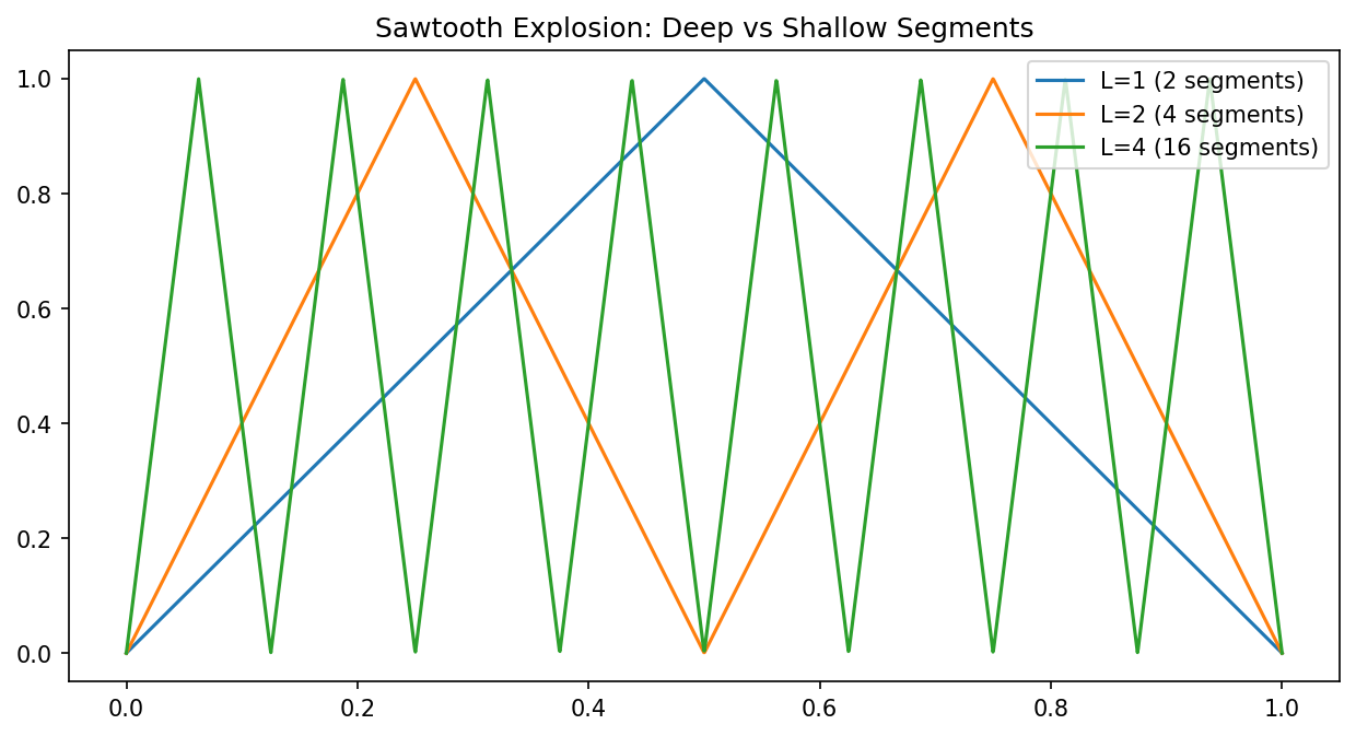
Demo 7.1: The Sawtooth Explosion
import matplotlib
matplotlib.use('Agg')
import torch
import matplotlib.pyplot as plt

def g(x): return torch.relu(2*x) - 2*torch.relu(2*x-1) + torch.relu(2*x-2)

x = torch.linspace(0, 1, 2000)
f1 = g(x)
f2 = g(f1)
f4 = g(g(f2))

plt.figure(figsize=(10, 5))
plt.plot(x.numpy(), f1.numpy(), label='L=1 (2 segments)')
plt.plot(x.numpy(), f2.numpy(), label='L=2 (4 segments)')
plt.plot(x.numpy(), f4.numpy(), label='L=4 (16 segments)')
plt.title("Sawtooth Explosion: Deep vs Shallow Segments")
plt.legend()
plt.savefig('figures/02-2-demo1.png', dpi=150, bbox_inches='tight')
plt.close()
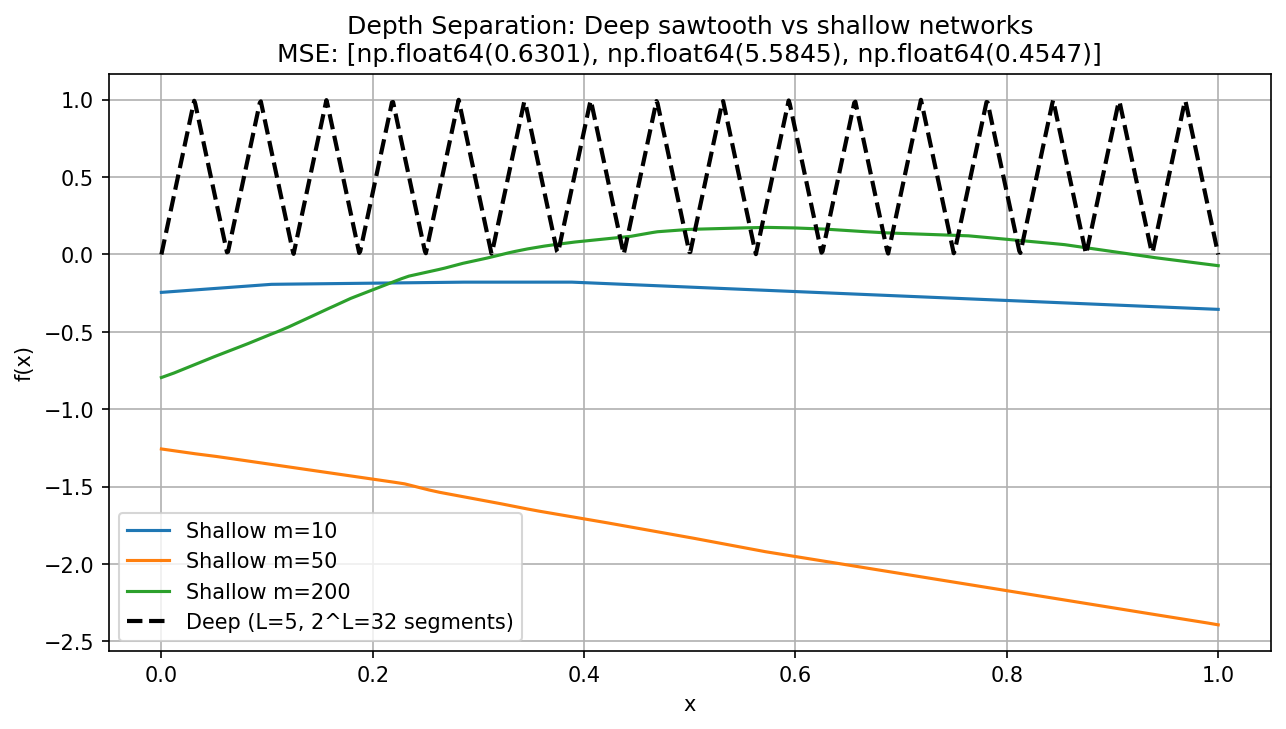
Demo 7.2: Empirical Training Comparison
import matplotlib
matplotlib.use('Agg')
import numpy as np
import matplotlib.pyplot as plt

def sawtooth(x, L):
    for _ in range(L):
        x = np.where(x < 0.5, 2*x, 2*(1-x))
    return x

def shallow_net(x, m=50):
    w = np.random.randn(m) * 2
    b = np.random.randn(m)
    v = np.random.randn(m) * 0.1
    return v @ np.maximum(0, w * x.reshape(-1, 1) + b).T

L = 5
x = np.linspace(0, 1, 1000)
y_deep = sawtooth(x.copy(), L)

mse_values = []
widths = [10, 50, 200]
plt.figure(figsize=(10, 5))
for m in widths:
    y_shallow = shallow_net(x, m)
    mse_values.append(np.mean((y_deep - y_shallow)**2))
    plt.plot(x, y_shallow, label=f'Shallow m={m}')

plt.plot(x, y_deep, 'k--', linewidth=2, label=f'Deep (L={L}, 2^L={2**L} segments)')
plt.xlabel('x'); plt.ylabel('f(x)')
plt.title(f'Depth Separation: Deep sawtooth vs shallow networks\nMSE: {[round(v,4) for v in mse_values]}')
plt.legend(); plt.grid(True)
plt.savefig('figures/02-2-demo2.png', dpi=150, bbox_inches='tight')
plt.close()
8. Conclusion
Depth separation theorems prove that the architecture of a neural network is not just a detail—it is a fundamental constraint on its representational efficiency. By leveraging hierarchy and composition, deep networks can compute functions that are topologically impossible for shallow networks of the same size.