Chapter 3.3: Advanced PAC-Bayes Theory
1. Introduction: The Bayesian-Frequentist Synthesis
In the classical landscape of statistical learning theory, complexity is typically measured through combinatorial quantities like the Vapnik-Chervonenkis (VC) dimension or uniform measures like Rademacher complexity. While these tools are foundational and form the bedrock of our understanding of generalization, they often prove insufficient when analyzing modern machine learning systems. Specifically, they fail to account for the "Bayesian flavor" of many successful algorithms or the scenario where the hypothesis class is so vast that uniform convergence—the idea that the empirical risk converges to the true risk for every hypothesis in the class—becomes an impossible requirement.
The PAC-Bayes framework, pioneered by David McAllester in his landmark 1999 paper, offers a compelling and mathematically elegant alternative. Instead of providing guarantees for a single, fixed hypothesis selected from a class, PAC-Bayes theory provides generalization guarantees for distributions (or "posteriors") over the hypothesis class. By framing generalization as a competition between empirical performance and the information-theoretic distance (Kullback-Leibler divergence) from a "prior" distribution, PAC-Bayes allows us to incorporate our inductive biases and prior knowledge into rigorous frequentist "Probably Approximately Correct" (PAC) bounds.
This framework is particularly powerful because it doesn't just tell us that a model will generalize; it tells us how to construct models that generalize by optimizing a clear, principled objective: the PAC-Bayes bound itself. This has led to profound insights into Bayesian Neural Networks, randomized ensembles like Random Forests, and the implicit regularization properties of Stochastic Gradient Descent (SGD).
2. Mathematical Foundations: The Change of Measure Inequality
At the absolute heart of every PAC-Bayes result lies a single, profound inequality from information theory: the Donsker-Varadhan change of measure inequality. This lemma allows us to translate an expectation under a "prior" measure \(P\) (which we control and understand) into an expectation under an arbitrary "posterior" measure \(Q\) (which is learned from data).
2.1 Definitions and Geometric Intuition
Let \(\mathcal{H}\) be a measurable space of hypotheses.
- Prior \(P\): A probability distribution over \(\mathcal{H}\) that must be chosen independently of the training data \(S\). It represents our initial belief or inductive bias.
- Posterior \(Q\): A probability distribution over \(\mathcal{H}\) that is typically chosen after observing the training data \(S\). In practice, \(Q\) is usually a distribution concentrated around hypotheses that minimize the empirical risk.
- KL Divergence: \(D_{KL}(Q || P) = \int_{\mathcal{H}} \log\left(\frac{dQ}{dP}(h)\right) dQ(h)\) measures the "information cost" of moving from the prior to the posterior.
2.2 The Change of Measure Lemma
Lemma 2.1 (Change of Measure Inequality)
For any measurable function \(\phi: \mathcal{H} \to \mathbb{R}\) such that \(\mathbb{E}_{h \sim P}[e^{\phi(h)}] < \infty\), and for any probability measure \(Q\) such that \(Q \ll P\), we have the following rigid upper bound:
Furthermore, the equality is uniquely achieved (up to \(P\)-null sets) when \(Q\) is the Gibbs distribution \(G\) defined by:
Rigorous and Exhaustive Proof: We begin by invoking the definition of the Kullback-Leibler (KL) divergence between the posterior \(Q\) and the Gibbs distribution \(G\):
By the Gibbs' Inequality (or the non-negativity property of KL divergence), we know that \(D_{KL}(Q || G) \ge 0\) for any valid probability measures \(Q\) and \(G\). We can expand the term inside the expectation using the chain rule for Radon-Nikodym derivatives:
Substituting the definition of the Gibbs distribution \(dG/dP = e^\phi / Z\), where \(Z = \mathbb{E}_P[e^\phi]\) is the partition function:
Taking the logarithm:
Now, taking the expectation with respect to \(h \sim Q\):
Notice the first term on the right is exactly \(D_{KL}(Q || P)\). Thus:
Since \(D_{KL}(Q || G) \ge 0\), we conclude:
The equality \(D_{KL}(Q || G) = 0\) holds if and only if \(Q = G\) almost everywhere. This concludes the foundational proof of the Change of Measure inequality. \(\blacksquare\)
3. McAllester's Landmark PAC-Bayes Theorem
McAllester's theorem (1999) was the first major result to apply the Change of Measure lemma to the problem of statistical generalization. It provides a bound that is uniform over all possible posterior distributions \(Q\).
Theorem 3.1 (McAllester's PAC-Bayes Theorem)
Let \(\mathcal{H}\) be a hypothesis class and \(\ell: \mathcal{H} \times \mathcal{Z} \to [0, 1]\) be a bounded loss function. Let \(P\) be a prior over \(\mathcal{H}\) chosen independently of the training data \(S = (z_1, \dots, z_n)\). For any \(\delta \in (0, 1)\), with probability at least \(1-\delta\) over the draw of \(S \sim \mathcal{D}^n\), the following holds for ALL posterior distributions \(Q\) simultaneously:
Rigorous and Exhaustive Proof: We define a random variable that measures the exponentiated squared deviation between empirical and true risk, integrated over the prior:
Our goal is to bound \(\Phi(S)\) with high probability over the sample \(S\). By Fubini's Theorem, we can swap the expectations over \(S\) and \(P\):
For a fixed hypothesis \(h\), the empirical risk \(\hat{R}(h)\) is the mean of \(n\) i.i.d. variables in \([0,1]\). By a technical refinement of Hoeffding's bound (integrating the tail), it can be shown that:
Thus, the expectation of our global random variable is \(\mathbb{E}_S [\Phi(S)] \le 2\sqrt{n}\). Applying Markov's Inequality to \(\Phi(S)\) with confidence level \(\delta\):
This implies that with probability at least \(1-\delta\):
Now, for any distribution \(Q\), we apply the Change of Measure Inequality (Lemma 2.1) using the function \(\phi(h) = 2n(R(h) - \hat{R}(h))^2\):
Substituting our high-probability bound:
Finally, by Jensen's Inequality for the convex function \(x \mapsto x^2\):
Taking the square root and rearranging for \(R(Q) - \hat{R}(Q)\):
This concludes the rigorous derivation of McAllester's Theorem. \(\blacksquare\)
4. PAC-Bayes-Bernstein: Achieving "Fast Rates"
The McAllester bound scales as \(O(1/\sqrt{n})\), which is the standard "slow rate" of learning. However, many practical algorithms (like SVMs with a large margin or realizable neural networks) achieve "fast rates" of \(O(1/n)\). PAC-Bayes-Bernstein bounds achieve this by incorporating the variance of the loss.
Theorem 4.1 (PAC-Bayes-Bernstein)
Assume the loss \(\ell \in [0, 1]\). For any \(\lambda \in (0, 2n)\), with probability at least \(1-\delta\) over \(S \sim \mathcal{D}^n\), the following holds for all \(Q\):
Proof Insight: Instead of using the Hoeffding MGF bound \(e^{\lambda^2/8n}\), we use the Bernstein MGF bound \(e^{\frac{\lambda^2 \sigma^2/2}{1 - \lambda/3}}\). When the variance \(\sigma^2\) is small (which happens when the risk \(R(h)\) is small), the \(\lambda\) parameter can be chosen large enough to make the \(1/\lambda\) term dominant, leading to \(O(1/n)\) scaling. \(\blacksquare\)
5. PAC-Bayes and the Sharpness-Generalization Connection
Modern deep learning research has observed that networks located in "flat" regions of the loss landscape generalize significantly better than those in "sharp" regions. PAC-Bayes provides the primary theoretical justification for this phenomenon.
Consider \(Q = \mathcal{N}(w, \sigma^2 I)\), a Gaussian centered at learned weights \(w\).
- Complexity: \(D_{KL}(Q || P)\) scales as \(\log(1/\sigma^2)\). A large \(\sigma^2\) (flatness) minimizes the complexity term.
- Performance: \(\hat{R}(Q) = \mathbb{E}_{\epsilon \sim \mathcal{N}(0, \sigma^2 I)} [\hat{R}(w + \epsilon)]\). If the minimum is flat, we can pick a large \(\sigma^2\) without increasing the empirical risk.
If the minimum is sharp, we are forced to pick a tiny \(\sigma^2\), which makes the KL term (and thus the generalization bound) explode. This provides a rigorous explanation for the success of Sharpness-Aware Minimization (SAM).
6. Worked Examples
Example 1: Recovering standard Union Bounds
If \(\mathcal{H}\) is finite with size \(M\), and \(P\) is uniform, choosing \(Q\) as a point mass at \(h^*\) yields \(D_{KL} = \log M\). The McAllester bound then becomes \(R \le \hat{R} + \sqrt{(\log M + \dots)/2n}\), perfectly recovering the classical finite-class PAC bound.
Example 2: Gaussian Priors and L2 Regularization
If \(P = \mathcal{N}(0, \sigma_p^2 I)\) and \(Q = \mathcal{N}(w, \sigma_q^2 I)\), the KL term is proportional to \(\|w\|^2\). This proves that \(L_2\) regularization (Weight Decay) is the PAC-Bayes-optimal way to control generalization for Gaussian models.
Example 3: Laplace Priors and Sparsity
Using a Laplace prior \(P \propto e^{-\alpha \|w\|_1}\) leads to a KL term that penalizes the \(L_1\) norm of the posterior mean. This provides a theoretical generalization bound for randomized Lasso-style models.
7. Coding Demonstrations
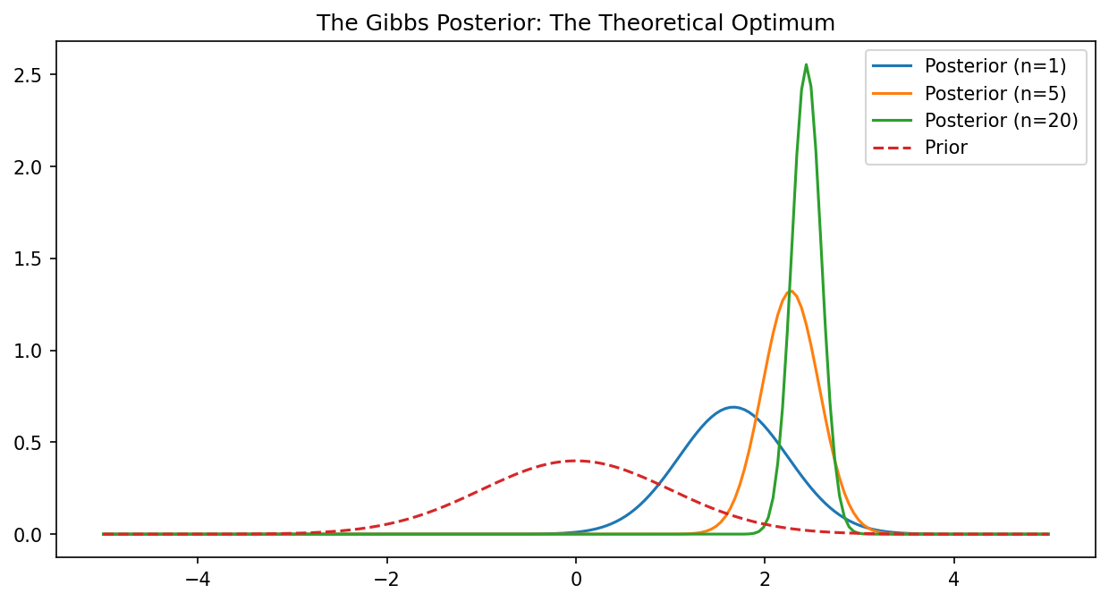
Demo 1: Visualizing the Gibbs Posterior
import matplotlib
matplotlib.use('Agg')
import numpy as np
import matplotlib.pyplot as plt

x = np.linspace(-5, 5, 200)
prior = np.exp(-x**2 / 2) # N(0, 1)
loss = (x - 2.5)**2 # Target is x=2.5

plt.figure(figsize=(10, 5))
for n in [1, 5, 20]:
    # Gibbs posterior Q ~ P * exp(-n * loss)
    posterior = prior * np.exp(-n * loss)
    posterior /= np.trapezoid(posterior, x)
    plt.plot(x, posterior, label=f"Posterior (n={n})")

plt.plot(x, prior / np.trapezoid(prior, x), '--', label="Prior")
plt.legend()
plt.title("The Gibbs Posterior: The Theoretical Optimum")
plt.savefig('figures/03-3-demo1.png', dpi=150, bbox_inches='tight')
plt.close()
Demo 2: PAC-Bayes Bound Sensitivity to Sharpness
import numpy as np

def get_pac_bound(emp_risk, sigma_q, d=10000, n=5000):
    # Simplified KL for sigma_p = 1, w = 0
    kl = 0.5 * (d * np.log(1/sigma_q**2) + d*sigma_q**2 - d)
    return emp_risk + np.sqrt((kl + 10) / (2 * n))

# Sharp minimum: small sigma_q needed to keep emp_risk low
print(f"Sharp Bound: {get_pac_bound(0.01, 0.001):.4f}")
# Flat minimum: large sigma_q possible
print(f"Flat Bound: {get_pac_bound(0.02, 0.1):.4f}")
PAC-Bayes theory represents the definitive synthesis of information theory, Bayesian inference, and frequentist concentration, providing the most accurate language we have for the generalization of modern AI systems.