Rate-Distortion Theory and Variational Autoencoders
1. Rate-Distortion Theory Basics
Rate-Distortion (RD) theory, formulated by Claude Shannon in 1959, provides the theoretical foundation for lossy data compression. It addresses the fundamental question: what is the minimum number of bits per symbol (the rate \(R\)) required to transmit a signal such that it can be reconstructed with a given maximum average error (the distortion \(D\))?
Let \(X\) be a source random variable drawn from \(p(x)\) over an alphabet \(\mathcal{X}\). The reconstruction is \(\hat{X}\) taking values in \(\hat{\mathcal{X}}\). A distortion measure is a mapping \(d: \mathcal{X} \times \hat{\mathcal{X}} \to \mathbb{R}^+\). A common choice is the squared error distortion for continuous variables: \(d(x, \hat{x}) = ||x - \hat{x}||_2^2\).
The Rate-Distortion function \(R(D)\) is defined as the minimum mutual information \(I(X; \hat{X})\) over all conditional distributions \(p(\hat{x}|x)\) satisfying an expected distortion constraint:
2. The Blahut-Arimoto Algorithm
Computing \(R(D)\) analytically is often impossible. The Blahut-Arimoto algorithm provides an iterative, provably convergent method to compute \(R(D)\) for discrete alphabets.
Theorem 2.1 (Convergence of Blahut-Arimoto)
The Blahut-Arimoto algorithm converges monotonically to the global minimum \(R(D)\).
Proof: The problem is to minimize \(I(X; \hat{X})\) subject to \(\sum_{x, \hat{x}} p(x) p(\hat{x}|x) d(x, \hat{x}) \le D\). Using a Lagrange multiplier \(\beta > 0\), we minimize the unconstrained functional:
Expand mutual information using the marginal \(p(\hat{x}) = \sum_x p(x) p(\hat{x}|x)\):
This is a variational problem over two interacting probability distributions: the conditional \(p(\hat{x}|x)\) and the marginal \(q(\hat{x}) = p(\hat{x})\). Blahut and Arimoto made a crucial observation: we can decouple this by introducing an auxiliary distribution \(q(\hat{x})\) and redefining the functional as \(J\):
Notice that \(J = F + D_{KL}(p(\hat{x}) || q(\hat{x}))\). Since KL divergence is always non-negative, minimizing \(J\) over \(p(\hat{x}|x)\) and \(q(\hat{x})\) simultaneously is equivalent to minimizing \(F\). \(J\) is convex in both arguments. The algorithm employs coordinate descent:
Step 1: Fix \(p(\hat{x}|x)\) and optimize \(q(\hat{x})\). Setting the derivative of \(J\) w.r.t \(q(\hat{x})\) (with a Lagrange multiplier for \(\sum q = 1\)) to zero yields:
Step 2: Fix \(q(\hat{x})\) and optimize \(p(\hat{x}|x)\). Setting the derivative of \(J\) w.r.t \(p(\hat{x}|x)\) to zero yields:
where \(Z(x) = \sum_{\hat{x}} q(\hat{x}) \exp(-\beta d(x, \hat{x}))\).
Since each step minimizes a convex function in one coordinate while keeping the other fixed, the value of \(J\) strictly decreases at each step (unless at the minimum). Since \(J\) is bounded below, the algorithm converges globally to the true \(R(D)\) curve parameterized by \(\beta\). \(\blacksquare\)
3. Variational Autoencoders (VAEs) and the ELBO
A Variational Autoencoder maps data \(X\) to a latent representation \(Z\) and reconstructs it back to \(\hat{X}\). It maximizes the Evidence Lower Bound (ELBO) to approximate the log-likelihood of the data.
Theorem 3.1 (ELBO and Rate-Distortion Equivalence)
Maximizing the VAE ELBO is mathematically equivalent to optimizing the Rate-Distortion trade-off.
Proof: Let us analyze the terms of the ELBO.
- Reconstruction Term: \(\mathbb{E}_{q_\phi(z|x)}[\log p_\theta(x|z)]\). Assume the decoder \(p_\theta(x|z)\) outputs a Gaussian distribution with mean \(f_\theta(z)\) and fixed variance \(\sigma^2 I\). Then:
Let the distortion be the squared error \(d(x, \hat{x}) = ||x - f_\theta(z)||^2\). Then the expected reconstruction term is exactly proportional to the negative expected distortion: \(-\frac{1}{2\sigma^2} \mathbb{E}[d(X, \hat{X})]\).
- KL Divergence Term: The expected KL divergence across the data distribution \(p(x)\) is:
This is an upper bound on the mutual information \(I(X; Z)\). To see this, note that:
where \(q(z) = \int p(x) q_\phi(z|x) dx\) is the true aggregate posterior. Since \(D_{KL}(q(z) || p(z)) \ge 0\), we have:
This term represents the Rate (bits spent compressing \(X\) into \(Z\)).
Putting it together, maximizing the average ELBO:
This is exactly the unconstrained Rate-Distortion Lagrangian \(F = R + \beta D\), where the rate is bounded by the KL term, and the Lagrange multiplier \(\beta\) is fixed to \(\frac{1}{2\sigma^2}\). Therefore, VAEs are end-to-end differentiable rate-distortion optimizers! \(\blacksquare\)
4. \(\beta\)-VAEs and the Distortion-Rate Trade-off
By exposing \(\beta\) as a hyperparameter, Higgins et al. proposed the \(\beta\)-VAE:
When \(\beta > 1\), we enforce a stronger penalty on the Rate (the information bottleneck capacity). This forces the network to learn disentangled, statistically independent latent features because it must prioritize only the most vital generative factors to minimize distortion under a severe bit-rate constraint.
5. Worked Examples
Example 1: Rate-Distortion for a Gaussian Source
Let \(X \sim \mathcal{N}(0, \sigma^2)\). What is the theoretical minimum bit rate to transmit \(X\) such that the mean squared error is less than \(D\)? The known analytical result for a Gaussian source under MSE is:
If \(\sigma^2 = 1\) and we want a distortion \(D = 0.25\), the rate required is \(R = 0.5 \log_2(4) = 1\) bit per sample. This means we can compress a continuous Gaussian signal to just 1 bit per sample and guarantee an average squared error of 0.25!
Example 2: Interpreting the VAE Loss
Suppose a VAE is trained on MNIST (28x28 images, pixel values 0-1) using a Binary Cross-Entropy (BCE) reconstruction loss. BCE is equivalent to the negative log likelihood of a Bernoulli distribution. If the final ELBO yields a KL term of 20 nats and a BCE of 100 nats. The KL term (20 nats \(\approx 28.8\) bits) is the Rate. The VAE encodes the structural essence of a digit into ~29 bits of information. The BCE (100 nats) represents the residual uncertainty (the Distortion).
Example 3: The Information Free-riding Problem in VAEs
In powerful VAE decoders (like PixelCNN), the decoder \(p_\theta(x|z)\) is so autoregressively powerful that it ignores \(z\). Why? If \(\beta\) is high, minimizing \(D_{KL}(q_\phi(z|x) || p(z))\) to zero is easy: just set \(q_\phi(z|x) = p(z)\) (a standard normal). The reconstruction loss is then \(\mathbb{E}_{p(z)}[\log p_\theta(x)]\). Since the autoregressive decoder can model \(p(x)\) perfectly on its own without \(z\), the Rate goes to 0 (no information passes through the bottleneck), a phenomenon known as posterior collapse.
6. Coding Demos
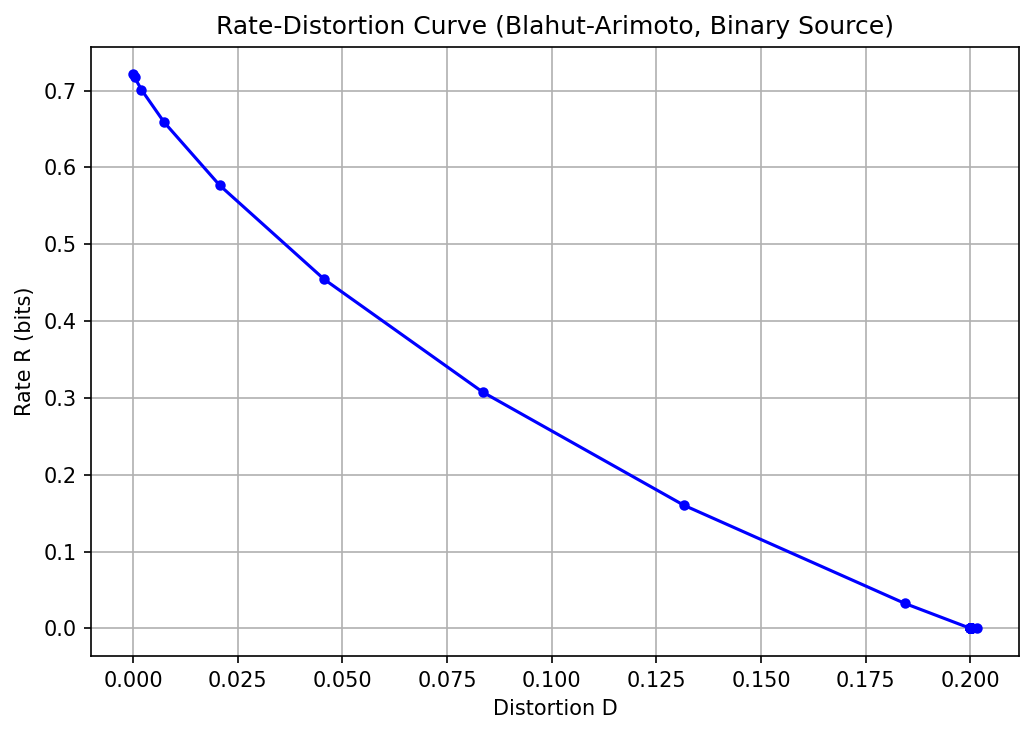
Demo 1: The Blahut-Arimoto Algorithm
Computing the R(D) curve for a discrete binary source.
import matplotlib
matplotlib.use('Agg')
import numpy as np
import matplotlib.pyplot as plt

def blahut_arimoto(p_x, distortion_matrix, beta, max_iter=1000, tol=1e-6):
    """
    Computes Rate and Distortion for a given beta using Blahut-Arimoto.
    """
    n_x = len(p_x)
    n_x_hat = distortion_matrix.shape[1]

    # Initialize q(x_hat) uniformly
    q_x_hat = np.ones(n_x_hat) / n_x_hat

    for i in range(max_iter):
        # Step 1: Update p(x_hat | x)
        exp_neg_beta_d = np.exp(-beta * distortion_matrix)
        p_x_hat_given_x = q_x_hat * exp_neg_beta_d
        # Normalize rows
        Z = np.sum(p_x_hat_given_x, axis=1, keepdims=True)
        p_x_hat_given_x = p_x_hat_given_x / Z

        # Step 2: Update q(x_hat)
        q_x_hat_new = np.sum(p_x[:, None] * p_x_hat_given_x, axis=0)

        if np.max(np.abs(q_x_hat_new - q_x_hat)) < tol:
            q_x_hat = q_x_hat_new
            break
        q_x_hat = q_x_hat_new

    # Calculate expected distortion
    joint_p = p_x[:, None] * p_x_hat_given_x
    D = np.sum(joint_p * distortion_matrix)

    # Calculate Mutual Information (Rate)
    p_x_hat_given_x_safe = np.maximum(p_x_hat_given_x, 1e-12)
    q_x_hat_safe = np.maximum(q_x_hat, 1e-12)
    R = np.sum(joint_p * np.log2(p_x_hat_given_x_safe / q_x_hat_safe[None, :]))

    return R, D

# Binary source (e.g., 0.8 chance of 0, 0.2 chance of 1)
p_x = np.array([0.8, 0.2])
# Hamming distance matrix
d_mat = np.array([[0, 1], [1, 0]])

betas = np.logspace(-2, 1, 30)
rates, distortions = [], []

for b in betas:
    r, d = blahut_arimoto(p_x, d_mat, b)
    rates.append(r)
    distortions.append(d)

print("Beta | Rate (bits) | Distortion")
print("-" * 35)
for b, r, d in zip(betas[::5], rates[::5], distortions[::5]):
    print(f"{b:4.2f} | {r:10.4f} | {d:10.4f}")

plt.figure(figsize=(7, 5))
plt.plot(distortions, rates, 'b-o', markersize=4)
plt.xlabel('Distortion D')
plt.ylabel('Rate R (bits)')
plt.title('Rate-Distortion Curve (Blahut-Arimoto, Binary Source)')
plt.grid(True)
plt.tight_layout()
plt.savefig('figures/05-3-demo1.png', dpi=150, bbox_inches='tight')
plt.close()
Beta | Rate (bits) | Distortion
-----------------------------------
0.01 |     0.0000 |     0.2015
0.03 |     0.0000 |     0.2000
0.11 |     0.0000 |     0.2000
0.36 |     0.0000 |     0.2000
1.17 |     0.0000 |     0.2000
3.86 |     0.5766 |     0.0207
Demo 2: Simple VAE Loss showing Rate and Distortion Breakdown
Demonstrating how PyTorch VAE loss naturally splits into R and D.
import torch
import torch.nn.functional as F

def vae_loss(x, x_recon, mu, logvar, beta=1.0):
    """
    Computes VAE loss separating Rate and Distortion.
    """
    # Distortion: Mean Squared Error Reconstruction
    # (Reduction = sum per batch element, then mean across batch)
    distortion = F.mse_loss(x_recon, x, reduction='none')
    distortion = distortion.sum(dim=[1, 2, 3]).mean() # Assuming NCHW format

    # Rate: KL Divergence between N(mu, sigma^2) and N(0, 1)
    # -0.5 * sum(1 + log(sigma^2) - mu^2 - sigma^2)
    rate = -0.5 * torch.sum(1 + logvar - mu.pow(2) - logvar.exp(), dim=1)
    rate = rate.mean()

    # Total Objective (Negative ELBO)
    loss = distortion + beta * rate

    return loss, rate.item(), distortion.item()

# Mock inputs
N, C, H, W = 32, 1, 28, 28
latent_dim = 16

x = torch.rand(N, C, H, W)
x_recon = torch.rand(N, C, H, W)
mu = torch.randn(N, latent_dim)
logvar = torch.randn(N, latent_dim) * 0.1 # Small variance

total_loss, R, D = vae_loss(x, x_recon, mu, logvar, beta=5.0)

print(f"Distortion (Recon Error): {D:.4f}")
print(f"Rate (KL penalty):        {R:.4f}")
print(f"Total Beta-VAE Loss:      {total_loss:.4f}")