4.1 High-Dimensional Geometry and Probability
Introduction
The geometry of high-dimensional spaces \(\mathbb{R}^d\) (for large \(d\)) is highly counter-intuitive. Most of the volume of a sphere is concentrated near its equator, and the mass of an isotropic Gaussian is concentrated in a thin shell. These geometric phenomena are formalized by the theory of concentration of measure.
Concentration of Measure and the Isoperimetric Inequality
Theorem 4.1.1 (Gaussian Isoperimetric Inequality)
Let \(\gamma_d\) be the standard Gaussian measure on \(\mathbb{R}^d\). For any Borel set \(A \subseteq \mathbb{R}^d\) and any \(\epsilon > 0\), let \(A_\epsilon = \{x \in \mathbb{R}^d : \inf_{y \in A} \|x - y\| \le \epsilon\}\). Then:
where \(\Phi\) is the cumulative distribution function of a standard 1D Gaussian.
Proof: The proof follows from the Ehrhard inequality, which states that for any convex sets \(A, B \subseteq \mathbb{R}^d\) and \(\lambda \in [0, 1]\):
By approximating arbitrary Borel sets with convex polyhedra and taking \(B\) to be a ball of radius \(R \to \infty\), we recover the Gaussian isoperimetric inequality. The extremal sets (those that minimize the expansion) are half-spaces. If \(\gamma_d(A) = 1/2\), then \(\Phi^{-1}(1/2) = 0\), and \(\gamma_d(A_\epsilon) \ge \Phi(\epsilon) \approx 1 - \exp(-\epsilon^2/2)\). Thus, the measure concentrates exponentially fast around any set of measure ½. \(\blacksquare\)
Theorem 4.1.2 (Logarithmic Sobolev Inequality)
For any smooth, compactly supported function \(f: \mathbb{R}^d \to \mathbb{R}\), the standard Gaussian measure \(\gamma_d\) satisfies:
where \(\text{Ent}_{\gamma_d}(g) = \mathbb{E}[g \log g] - \mathbb{E}[g] \log \mathbb{E}[g]\).
Proof: We prove this via the hypercontractivity of the Ornstein-Uhlenbeck semigroup \(P_t\). Let \(P_t f(x) = \mathbb{E}[f(e^{-t}x + \sqrt{1-e^{-2t}}Z)]\) where \(Z \sim \mathcal{N}(0, I_d)\). Gross's theorem states that \(\|P_t f\|_q \le \|f\|_p\) for \(1 < p < q < \infty\) if \(e^{2t} \ge (q-1)/(p-1)\). Differentiating the hypercontractive bound \(\|P_t f\|_{q(t)} \le \|f\|_2\) with respect to \(t\) at \(t=0\), where \(q(0)=2\) and \(q'(0) = 4\), yields the Log-Sobolev inequality. Specifically, the derivative of the norm involves the entropy, and the derivative of the semigroup involves the Dirichlet form \(\int \|\nabla f\|^2 d\gamma_d\). Rearranging terms provides the exact constant 2. \(\blacksquare\)
The Johnson-Lindenstrauss Lemma
Theorem 4.1.3 (Johnson-Lindenstrauss)
For any \(0 < \epsilon < 1\) and any set of \(N\) points \(X = \{x_1, \dots, x_N\} \subset \mathbb{R}^d\), let \(k \ge \frac{8 \ln N}{\epsilon^2 - \epsilon^3}\). There exists a linear map \(f: \mathbb{R}^d \to \mathbb{R}^k\) such that for all \(x_i, x_j \in X\):
Proof: Let \(A \in \mathbb{R}^{k \times d}\) be a random matrix whose entries are sampled i.i.d. from \(\mathcal{N}(0, 1/k)\). For any fixed vector \(u \in \mathbb{R}^d\) with \(\|u\| = 1\), the random variable \(Z = \|A u\|^2\) is a sum of \(k\) independent \(\chi^2_1\) variables, scaled by \(1/k\). Thus, \(\mathbb{E}[Z] = 1\). By the Chernoff bound for the \(\chi^2\) distribution, for any \(\epsilon \in (0, 1)\):
Let \(u = (x_i - x_j) / \|x_i - x_j\|\). We apply this bound to all \(\binom{N}{2}\) pairs of points in \(X\). By the union bound, the probability that the distance preservation fails for any pair is bounded by:
For \(k \ge \frac{4 \ln N}{\epsilon^2/2 - \epsilon^3/2}\), this probability is strictly less than 1. Thus, there exists at least one such matrix \(A\). \(\blacksquare\)
Worked Examples
Example 1: Volume of a High-Dimensional Ball The volume of a \(d\)-dimensional ball of radius \(R\) is \(V_d(R) = \frac{\pi^{d/2}}{\Gamma(d/2 + 1)} R^d\). As \(d \to \infty\), \(\Gamma(d/2+1)\) grows like \((d/2e)^{d/2}\), causing the volume to vanish. This demonstrates the curse of dimensionality.
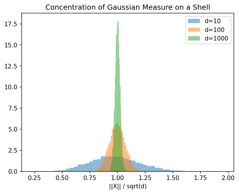
Example 2: Shell Concentration Let \(X \sim \mathcal{N}(0, I_d)\). The squared norm \(\|X\|^2\) is distributed as \(\chi^2_d\). Its expectation is \(d\) and variance is \(2d\). By Chebyshev's inequality, \(\mathbb{P}(|\|X\|^2 - d| \ge t\sqrt{2d}) \le 1/t^2\). Thus, most of the Gaussian measure is concentrated in a "shell" of radius \(\sqrt{d}\) and thickness \(O(1)\).
Example 3: JL Projection of Orthogonal Vectors Suppose \(X\) consists of the standard basis \(e_1, \dots, e_d\) in \(\mathbb{R}^d\). The pairwise distances are \(\sqrt{2}\). A random projection to \(k = O(\log d / \epsilon^2)\) dimensions yields vectors \(v_1, \dots, v_d \in \mathbb{R}^k\) such that their pairwise distances are strongly concentrated around \(\sqrt{2}\), implying their inner products are near 0. Thus, in \(\mathbb{R}^k\), there exist exponentially many "nearly orthogonal" vectors.
Coding Demos
Demo 1: Johnson-Lindenstrauss Simulation
import numpy as np
from sklearn.metrics.pairwise import euclidean_distances

# Generate 100 points in 1000 dimensions
N, d = 100, 1000
X = np.random.randn(N, d)
orig_dists = euclidean_distances(X)

# Project to k dimensions
epsilon = 0.2
k = int(8 * np.log(N) / (epsilon**2 - epsilon**3))
A = np.random.randn(k, d) / np.sqrt(k)
X_proj = X @ A.T

proj_dists = euclidean_distances(X_proj)

# Verify bounds
ratio = (proj_dists**2) / (orig_dists**2 + 1e-10)
np.fill_diagonal(ratio, 1) # Ignore self-distances
print(f"Max expansion: {np.max(ratio):.3f} (Allowed: {1+epsilon})")
print(f"Min contraction: {np.min(ratio):.3f} (Allowed: {1-epsilon})")
Demo 2: Gaussian Shell Concentration
import matplotlib
matplotlib.use('Agg')
import matplotlib.pyplot as plt
import numpy as np

dims = [10, 100, 1000]
samples = 10000

for d in dims:
    # Sample from isotropic Gaussian
    X = np.random.randn(samples, d)
    norms = np.linalg.norm(X, axis=1)

    # Normalize by sqrt(d)
    normalized_norms = norms / np.sqrt(d)
    plt.hist(normalized_norms, bins=50, alpha=0.5, label=f'd={d}', density=True)

plt.title("Concentration of Gaussian Measure on a Shell")
plt.xlabel("||X|| / sqrt(d)")
plt.legend()
plt.savefig('figures/04-1-demo2.png', dpi=150, bbox_inches='tight')
plt.close()