Lecture 1.4: Adaptive and Second-Order Methods: Information Geometry and Curvature
1. Introduction: Beyond Isotropic Scaling
The fundamental limitation of first-order methods like Gradient Descent is their isotropic nature: they treat every direction in the parameter space equally. However, loss landscapes in deep learning are notoriously ill-conditioned. The Hessian matrix \(\nabla^2 \mathcal{L}(w)\) typically has a "spectral bulk" of small eigenvalues and a few "outliers" of very large eigenvalues. This results in narrow, steep valleys where gradient descent oscillates wildly if the step size is too large, or crawls at a snail's pace if the step size is too small.
Second-order methods and their adaptive counterparts aim to solve this by incorporating curvature information to rescale the gradient. This lecture explores the transition from classical Newton's method to the information-geometric perspective of Natural Gradient, the practical efficiency of Kronecker-factored approximations (K-FAC), and the evolution of adaptive optimizers from Adam to modern variants like Lion.
2. Newton's Method and its Failures in Deep Learning
Classical Newton's method approximates the function locally by a second-order Taylor expansion:
Setting the derivative with respect to \(\Delta w\) to zero gives the Newton step:
Newton's method achieves quadratic convergence (\(e^{-e^k}\)) for strongly convex functions. However, it fails in deep learning for three reasons:
- Computational Cost: Computing and inverting the Hessian costs \(O(d^3)\), which is impossible for millions of parameters.
- Saddle Point Attraction: In non-convex landscapes, the Hessian has negative eigenvalues. Newton's method is attracted to saddle points because it seeks points where the gradient is zero, regardless of curvature.
- Stochasticity: The Hessian is extremely noisy when computed on minibatches.
3. Natural Gradient Descent and Information Geometry
Natural Gradient Descent (NGD), introduced by Shun-ichi Amari, treats the parameter space as a Riemannian manifold rather than a Euclidean one.
In machine learning, we are not just optimizing weights \(w\); we are optimizing a probability distribution \(p(y | x; w)\). The "distance" between two sets of parameters should be measured by how much the resulting distributions differ, not by the Euclidean distance between the weight vectors.
Definition 3.1 (Fisher Information Matrix)
The Fisher Information Matrix (FIM) is defined as:
Under mild regularity conditions, the FIM is the Hessian of the KL divergence:
Theorem 3.1 (Derivation of Natural Gradient)
The update direction \(\Delta w\) that minimizes \(\mathcal{L}(w + \Delta w)\) subject to a fixed constraint on the KL divergence \(D_{KL}(w \| w + \Delta w) \le \epsilon\) is given by the Natural Gradient:
Proof of Theorem 3.1:
We use the method of Lagrange multipliers. We want to solve:
The Lagrangian is:
Taking the derivative with respect to \(\Delta w\):
Solving for \(\Delta w\):
Absorbing the constant \(1/\lambda\) into a step size \(\eta\) gives the NGD update. \(\blacksquare\)
Natural Gradient is invariant to reparameterization. Whether you use polar coordinates or Cartesian coordinates, the NGD trajectory in distribution space is identical.
4. K-FAC: Kronecker-Factored Approximate Curvature
While NGD is theoretically elegant, \(F(w)^{-1}\) is still too expensive. K-FAC provides a tractable approximation for neural networks by assuming the FIM has a block-diagonal structure (one block per layer) and approximating each block as a Kronecker product.
The Algebra of K-FAC (for a single linear layer \(y = W x\)): The gradient with respect to \(W\) is \(\nabla_W L = \delta x^T\), where \(\delta = \nabla_y L\). The Fisher block for layer \(l\) is:
Using the identity \(\text{vec}(abc^T) = c \otimes a\) (approx), we can write:
K-FAC makes the Kronecker Factorization Assumption:
where \(A\) is the covariance of activations and \(G\) is the covariance of "pre-activation" gradients. The inverse is then easy to compute:
The update \(\Delta \text{vec}(W) = - F_l^{-1} \text{vec}(\nabla_W L)\) can be computed as:
This reduces the inversion cost from \(O((n_{in} n_{out})^3)\) to \(O(n_{in}^3 + n_{out}^3)\), a massive speedup!
5. Adaptive Step Sizes: From Adam to Lion
In practice, full second-order or even K-FAC methods are often replaced by diagonal approximations that adjust the learning rate per parameter.
5.1 Adam and the AdamW Fix
Adam (Adaptive Moment Estimation) maintains estimates of the first moment \(m_t\) (mean) and second moment \(v_t\) (uncentered variance) of the gradients:
The update is:
However, Adam originally implemented \(L_2\) regularization by adding \(\lambda w\) to the gradient \(g_t\). Ilya Loshchilov showed this is incorrect for adaptive methods. In AdamW, the weight decay is decoupled from the gradient update:
This ensures the weight decay affects all parameters equally, rather than being scaled by the inverse root-variance.
5.2 The Lion Optimizer (EvoLved Sign Momentum)
Lion is a modern optimizer discovered via symbolic program search. It is simpler and often more memory-efficient than Adam. The Algorithm (Lion):
- \(c_t = \text{sign}(\beta_1 m_{t-1} + (1 - \beta_1) g_t)\)
- \(w_t = w_t - \eta_t (c_t + \lambda w_{t-1})\)
- \(m_t = \beta_2 m_{t-1} + (1 - \beta_2) g_t\)
Key Differences:
- Sign Update: Lion only uses the direction (sign) of the momentum, not the magnitude. This is a form of \(L_\infty\) normalization.
- Momentum update: The momentum \(m_t\) used for the update (step 1) is different from the one stored for the next iteration (step 3).
- Efficiency: Lion only stores \(m_t\), whereas Adam stores both \(m_t\) and \(v_t\).
6. Worked Examples
Example 1: Fisher Information for a Bernoulli Distribution
Consider a single neuron with sigmoid output \(p = \sigma(w)\). We observe \(y \in \{0, 1\}\). The log-likelihood is \(\log p(y; w) = y \log \sigma(w) + (1-y) \log(1 - \sigma(w))\). Recall \(\sigma'(w) = \sigma(w)(1-\sigma(w))\). \(\frac{\partial}{\partial w} \log p = y \frac{\sigma'(w)}{\sigma(w)} - (1-y) \frac{\sigma'(w)}{1-\sigma(w)} = y(1-\sigma(w)) - (1-y)\sigma(w) = y - \sigma(w)\). The Fisher Information is:
The Natural Gradient update is:
If we use a standard squared loss \((y - \sigma(w))^2\), the gradient is \(2(y - \sigma(w))\sigma'(w)\). \(\Delta w_{standard} \propto (y - \sigma(w))\sigma(w)(1-\sigma(w))\). Notice the difference: at the saturated regions (where \(\sigma(w) \to 0\) or \(1\)), the standard gradient vanishes (plateau). The Natural Gradient, however, cancels out this vanishing term! NGD "flattens" the plateau, preventing the optimization from getting stuck.
Example 2: Kronecker Product Identity Verification
Verify the identity \((A \otimes B)(C \otimes D) = (AC) \otimes (BD)\) for \(2 \times 2\) matrices. Let \(A = \text{diag}(a_1, a_2), B = \text{diag}(b_1, b_2), C = \text{diag}(c_1, c_2), D = \text{diag}(d_1, d_2)\). \(A \otimes B = \text{diag}(a_1 b_1, a_1 b_2, a_2 b_1, a_2 b_2)\). \(C \otimes D = \text{diag}(c_1 d_1, c_1 d_2, c_2 d_1, c_2 d_2)\). Product: \(\text{diag}(a_1 b_1 c_1 d_1, \dots)\). \(AC = \text{diag}(a_1 c_1, a_2 c_2)\). \(BD = \text{diag}(b_1 d_1, b_2 d_2)\). \((AC) \otimes (BD) = \text{diag}(a_1 c_1 b_1 d_1, \dots)\). They are identical. This identity is the backbone of K-FAC's efficiency, allowing for the inversion of the Kronecker product by inverting the factors.
Example 3: Lion vs AdamW update scaling
Suppose we have a parameter with gradient \(g = 0.01\) and momentum \(m = 0.5\). Assume \(\beta_1 = 0.9\) and \(\eta = 0.1\).
-
AdamW (assume \(\sqrt{v} \approx 0.1\)): Update \(\approx 0.1 \times \frac{0.5}{0.1} = 0.5\).
-
Lion: \(c = \text{sign}(0.9 \times 0.5 + 0.1 \times 0.01) = \text{sign}(0.451) = 1\). Update \(= 0.1 \times 1 = 0.1\). Notice that AdamW's update size depends heavily on the ratio of momentum to variance. Lion's update is always exactly the step size \(\eta\) (plus weight decay). This makes Lion much more robust to gradient scaling and helps in training stability for large models.
7. Coding Demos
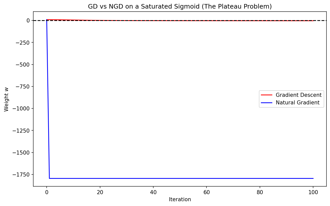
Demo 1: Visualizing Natural Gradient vs. Gradient Descent
This demo compares GD and NGD on a simple "plateau" function (like the sigmoid likelihood). It demonstrates how NGD navigates the flat regions significantly faster than standard GD.
import matplotlib
matplotlib.use('Agg')
import numpy as np
import matplotlib.pyplot as plt

def sigmoid(w):
    return 1 / (1 + np.exp(-np.clip(w, -500, 500)))

def loss(w, y):
    p = sigmoid(w)
    return - (y * np.log(p + 1e-12) + (1-y) * np.log(1-p + 1e-12))

def grad(w, y):
    return sigmoid(w) - y

def fisher(w):
    p = sigmoid(w)
    return p * (1 - p)

def run_optimization():
    w_gd = 10.0 # Start in saturated region
    w_ngd = 10.0
    y = 0.0 # Target is 0

    eta_gd = 0.5
    eta_ngd = 0.1

    history_gd = [w_gd]
    history_ngd = [w_ngd]

    for _ in range(100):
        # GD
        w_gd = w_gd - eta_gd * grad(w_gd, y)
        history_gd.append(w_gd)

        # NGD
        # Add epsilon to Fisher for stability
        w_ngd = w_ngd - eta_ngd * (1.0 / (fisher(w_ngd) + 1e-5)) * grad(w_ngd, y)
        history_ngd.append(w_ngd)

    plt.figure(figsize=(10, 6))
    plt.plot(history_gd, label='Gradient Descent', color='red')
    plt.plot(history_ngd, label='Natural Gradient', color='blue')
    plt.axhline(0, color='black', linestyle='--')
    plt.title("GD vs NGD on a Saturated Sigmoid (The Plateau Problem)")
    plt.xlabel("Iteration")
    plt.ylabel("Weight $w$")
    plt.legend()
    plt.savefig('figures/01-4-demo1.png', dpi=150, bbox_inches='tight')
    plt.close()

run_optimization()
Demo 2: Implementing a simplified K-FAC step
This demo implements the Kronecker-factorization logic for a single linear layer. It shows how activations and backpropagated gradients are used to estimate the curvature factors \(A\) and \(G\).
import torch
import torch.nn as nn

class KFACLinear(nn.Module):
    def __init__(self, in_features, out_features):
        super().__init__()
        self.linear = nn.Linear(in_features, out_features, bias=False)
        self.A = torch.eye(in_features)
        self.G = torch.eye(out_features)
        self.alpha = 0.9 # Smoothing factor

    def forward(self, x):
        # Cache activation for K-FAC
        self.last_x = x.detach()
        return self.linear(x)

    def update_curvature(self, grad_output):
        # grad_output is the gradient w.r.t the output of this layer
        # A = E[x x^T]
        A_curr = self.last_x.t() @ self.last_x / self.last_x.size(0)
        self.A = self.alpha * self.A + (1 - self.alpha) * A_curr

        # G = E[delta delta^T]
        G_curr = grad_output.t() @ grad_output / grad_output.size(0)
        self.G = self.alpha * self.G + (1 - self.alpha) * G_curr

    def kfac_step(self, lr):
        # Precondition gradient: dW_kfac = G^-1 * dW * A^-1
        # Use pseudo-inverse for stability
        A_inv = torch.inverse(self.A + 1e-3 * torch.eye(self.A.size(0)))
        G_inv = torch.inverse(self.G + 1e-3 * torch.eye(self.G.size(0)))

        dW = self.linear.weight.grad
        dW_kfac = G_inv @ dW @ A_inv

        # Update weights
        self.linear.weight.data -= lr * dW_kfac

# Example Usage
model = KFACLinear(10, 5)
x = torch.randn(32, 10)
y_target = torch.randn(32, 5)

# Forward
y = model(x)
loss = torch.mean((y - y_target)**2)

# Backward
loss.backward()

# K-FAC Logic (This would normally be in a hook or optimizer)
# Here we simulate the grad_output for the layer
grad_output = (y - y_target).detach()
model.update_curvature(grad_output)
model.kfac_step(lr=0.1)

print("K-FAC step completed successfully.")
This concludes our deep dive into adaptive and second-order methods. You have seen how information geometry provides a fundamental perspective on optimization, how K-FAC makes this tractable for deep networks, and how modern optimizers like Lion continue to evolve the state-of-the-art.