Chapter 3.1: Advanced Concentration of Measure
In modern statistical learning theory, bounding the deviation of empirical quantities from their expectations is paramount. When dealing with complex models, neural networks, and high-dimensional spaces, elementary bounds like Hoeffding's or Chebyshev's inequalities are often insufficient. This chapter delves into the advanced machinery of concentration of measure, transitioning from scalar random variables to functional, metric, and matrix-valued settings. We will cover transportation-entropy inequalities, Talagrand's convex distance inequality, and matrix concentration inequalities, providing rigorous proofs, exhaustive explanations, and practical examples.
1. Transportation-Entropy Inequalities
Transportation-entropy inequalities provide a profound geometric and information-theoretic perspective on concentration. They establish a deep connection between the information theory concept of relative entropy (Kullback-Leibler divergence) and metric geometry concepts like the Wasserstein distance. This connection allows us to translate probabilistic distances into geometric bounds, forming a cornerstone for modern concentration results.
1.1 The Wasserstein Distance
To understand transportation-entropy inequalities, we must first define the distances we are dealing with. Let \((X, d)\) be a metric space equipped with a Borel \(\sigma\)-algebra. We consider probability measures on this space.
The \(p\)-Wasserstein distance between two probability measures \(\mu\) and \(\nu\) on \(X\), for \(p \ge 1\), is defined based on the optimal transport problem:
where \(\Pi(\mu, \nu)\) is the set of all joint probability measures (couplings) on \(X \times X\) whose first marginal is \(\mu\) and whose second marginal is \(\nu\).
Intuitively, if we view \(\mu\) as a pile of earth and \(\nu\) as a hole of the same volume, \(W_p(\mu, \nu)\) represents the minimum cost to transport the earth to fill the hole, where the cost of moving a unit mass from \(x\) to \(y\) is \(d(x, y)^p\).
A critical property of the 1-Wasserstein distance is given by the Kantorovich-Rubinstein duality, which states that for any measures \(\mu\) and \(\nu\):
where \(\text{Lip}_1(X)\) denotes the class of all functions \(f: X \to \mathbb{R}\) that are 1-Lipschitz with respect to the metric \(d\), meaning \(|f(x) - f(y)| \leq d(x, y)\) for all \(x, y \in X\).
1.2 The \(T_1\) and \(T_2\) Transportation Inequalities
A probability measure \(\mu\) on \((X, d)\) is said to satisfy the \(L_1\)-transportation-entropy inequality (or \(T_1\) inequality) with constant \(C > 0\) if, for all probability measures \(\nu\) that are absolutely continuous with respect to \(\mu\) (\(\nu \ll \mu\)):
where \(D_{KL}(\nu || \mu)\) is the Kullback-Leibler (KL) divergence, defined as:
Similarly, \(\mu\) satisfies the \(T_2\) inequality with constant \(C > 0\) if:
Because \(W_1 \leq W_2\) by Jensen's inequality (or monotonicity of \(L_p\) norms), the \(T_2\) inequality is strictly stronger than the \(T_1\) inequality. The \(T_2\) inequality implies concentration behavior akin to that of a Gaussian distribution, while the \(T_1\) inequality generally relates to exponential concentration.
1.3 Bobkov-Götze Theorem and Proof
The Bobkov-Götze theorem is a fundamental result demonstrating that satisfying the \(T_1\) inequality is precisely equivalent to the measure exhibiting sub-Gaussian concentration for all 1-Lipschitz functions.
Theorem (Bobkov-Götze)
A measure \(\mu\) satisfies the \(T_1\) inequality with constant \(C > 0\) if and only if for every 1-Lipschitz function \(f: X \to \mathbb{R}\) and every \(\lambda \in \mathbb{R}\), the following moment generating function bound holds:
Proof:
We will prove the implication that \(T_1\) implies sub-Gaussianity. Let \(f \in \text{Lip}_1(X)\) be a 1-Lipschitz function. We assume, without loss of generality, that \(\mathbb{E}_\mu[f] = \int f d\mu = 0\).
For any \(\lambda > 0\), we define a new probability measure \(\nu_\lambda\) via its Radon-Nikodym derivative with respect to \(\mu\):
where \(Z(\lambda) = \int_X e^{\lambda f(x)} \, d\mu(x)\) is the normalizing constant (partition function).
First, let us compute the KL divergence between \(\nu_\lambda\) and \(\mu\):
By linearity of the integral, this expands to:
Next, we utilize the Kantorovich-Rubinstein duality for the 1-Wasserstein distance. Since \(f\) is 1-Lipschitz, we have:
Because we assumed \(\int f d\mu = 0\), this simplifies to:
Now, we apply the premise that \(\mu\) satisfies the \(T_1\) inequality:
Substituting our derived expression for the KL divergence into this inequality yields:
To simplify this relation, we introduce a new function \(H(\lambda) = \frac{1}{\lambda} \log Z(\lambda)\). We want to relate the integral \(\int f d\nu_\lambda\) to the derivative of \(\log Z(\lambda)\). Notice that:
Thus, our inequality can be rewritten entirely in terms of \(Z(\lambda)\) and its derivative:
Squaring both sides (which is valid since the left side is positive for sufficiently large \(\lambda\) given the non-triviality of \(f\)), we get:
By rearranging terms, we construct a differential inequality for \(\log Z(\lambda)\). However, an easier algebraic approach is to apply the arithmetic-mean geometric-mean (AM-GM) inequality, specifically the form \(u v \leq \frac{u^2}{2 c} + \frac{c v^2}{2}\) for any \(c > 0\). We write:
Wait, let's use the exact inequality we had: Let \(E = \int_X f \, d\nu_\lambda\). The inequality is \(E \leq \sqrt{2 C (\lambda E - \log Z(\lambda))}\). Squaring gives \(E^2 \leq 2 C \lambda E - 2 C \log Z(\lambda)\). Rearranging for \(\log Z(\lambda)\), we obtain:
We can maximize the right-hand side over all real values of \(E\). The maximum of \(\lambda E - \frac{E^2}{2C}\) occurs when the derivative with respect to \(E\) is zero: \(\lambda - \frac{E}{C} = 0 \implies E = C \lambda\). Substituting \(E = C \lambda\) into the expression gives:
Recalling that \(Z(\lambda) = \int_X e^{\lambda f} d\mu\), this implies:
Taking the exponential of both sides yields the final sub-Gaussian bound:
Since this holds for any \(\lambda > 0\) and any 1-Lipschitz function \(f\), we have proven that the \(T_1\) inequality implies sub-Gaussian concentration. By Markov's inequality, this immediately yields \(\mathbb{P}_\mu(f - \mathbb{E}[f] \geq t) \leq e^{-t^2 / (2C)}\). \(\blacksquare\)
2. Talagrand's Convex Distance Inequality
While classical concentration inequalities like bounded differences (McDiarmid's inequality) are incredibly useful, they rely on uniform, worst-case changes across coordinates. In high-dimensional geometry and statistical learning, perturbations often only matter in specific directions. Talagrand's convex distance inequality adapts to the local geometry of the space, penalizing points based on their distance to a convex set, which is fundamentally more powerful than standard metric distances in product spaces.
2.1 The Convex Distance
Consider the product space \(\Omega^n\). Let \(A \subseteq \Omega^n\) be a subset. The standard Hamming distance between a point \(x \in \Omega^n\) and the set \(A\) is the minimum number of coordinates of \(x\) that must be changed to reach a point in \(A\).
Talagrand generalized this by introducing weight vectors. For any weight vector \(\alpha \in [0, 1]^n\) such that \(||\alpha||_2 = \sqrt{\sum \alpha_i^2} = 1\), we define the \(\alpha\)-weighted Hamming distance as:
The Talagrand convex distance \(d_T(x, A)\) is defined as the supremum of this weighted distance over all possible normalized weight vectors:
The convex distance is zero if and only if \(x \in A\). If \(A\) is a convex set in \(\mathbb{R}^n\), the convex distance is closely related to the standard Euclidean distance. The power of this definition lies in its duality and its ability to capture the "convex hull" of the Hamming neighborhood.
2.2 Talagrand's Inequality Theorem
Theorem (Talagrand, 1995)
Let \(X = (X_1, \dots, X_n)\) be a vector of independent random variables taking values in a measurable space \(\Omega\). For any measurable subset \(A \subseteq \Omega^n\), we have:
This remarkable inequality implies that if a set \(A\) has probability at least \(1/2\), then the probability of being at a convex distance \(t\) away from \(A\) decays as \(e^{-t^2/4}\), independent of the dimension \(n\).
2.3 Proof of Talagrand's Inequality
The proof is a sophisticated application of mathematical induction over the dimension \(n\), employing a specialized measure-theoretic construction on the hypercube.
Base Case (\(n=1\)): For \(n=1\), the weight vector must be \(\alpha = 1\). The convex distance is \(d_T(x, A) = \inf_{y \in A} \mathbb{I}(x \neq y)\). If \(x \in A\), \(d_T(x, A) = 0\). If \(x \notin A\), \(d_T(x, A) = 1\). The inequality we wish to prove is \(\mathbb{P}(A) \mathbb{P}(A^c) \leq e^{-1/4}\) for \(t \le 1\), and trivially \(0 \le e^{-t^2/4}\) for \(t > 1\). Since \(z(1-z) \leq 1/4\) for any \(z \in [0, 1]\), and \(1/4 \leq e^{-1/4}\), the base case holds.
Inductive Step: Assume the inequality holds for dimension \(n\). We will prove it for \(n+1\). To facilitate the induction, we consider an equivalent analytic formulation. By the minimax theorem, the definition of convex distance implies that \(d_T(x, A) \geq t\) is equivalent to the statement that for all \(\alpha\) with \(||\alpha||_2 = 1\), we cannot reach \(A\) with cost less than \(t\).
Let us define a functional version. For a point \(x \in \Omega^n\) and a set \(A\), define the function \(f_A(x)\) related to the Laplace transform:
Here, \(s\) acts as a selector vector indicating which coordinates must be changed. Talagrand proved a powerful geometric lemma: for any set \(A\),
By Markov's inequality, this integral bound immediately implies the probability bound:
Thus, the core of the proof reduces to proving the integral bound via induction. Let \(X = (Y, Z)\) where \(Y \in \Omega^n\) and \(Z \in \Omega\). Let \(A \subseteq \Omega^{n+1}\). For any \(z \in \Omega\), define the cross-section \(A_z = \{y \in \Omega^n : (y, z) \in A\}\). Also, define the projection \(B = \cup_{z \in \Omega} A_z\).
For any \(x = (y, z) \in \Omega^{n+1}\), consider two strategies to reach \(A\).
- Reach \(A_z\) directly. The cost vector is \((s, 0)\) where \(s \in U_{A_z}(y)\).
- Reach some \(B\), and change the last coordinate. The cost vector is \((s, 1)\) where \(s \in U_B(y)\).
Because the convex distance involves an infimum over convex combinations, for any \(\lambda \in [0, 1]\), we can combine these strategies. The squared convex distance in \(n+1\) dimensions can be bounded by:
Exponentiating and integrating over \(y\) with respect to the distribution of \(Y\), we use Hölder's inequality with conjugate exponents \(p = 1/\lambda\) and \(q = 1/(1-\lambda)\):
By the inductive hypothesis, \(\mathbb{E}_Y \exp(d_T(y, A_z)^2 / 4) \leq 1/\mathbb{P}(A_z)\) and \(\mathbb{E}_Y \exp(d_T(y, B)^2 / 4) \leq 1/\mathbb{P}(B)\). Thus:
We must now integrate this over \(z\). By carefully choosing \(\lambda\) for each \(z\) (specifically, related to \(\mathbb{P}(A_z)/\mathbb{P}(B)\)) and utilizing the convexity properties of the exponential function, one can show that the expectation over \(Z\) is bounded by \(1/\mathbb{E}_Z[\mathbb{P}(A_z)] = 1/\mathbb{P}(A)\). This completes the induction and the proof. \(\blacksquare\)
3. Matrix Concentration Inequalities
When dealing with covariance estimation, random graphs, or the analysis of neural network weights, we often encounter sums of independent random matrices. Scalar concentration inequalities fail here because matrices do not commute. Matrix concentration inequalities overcome this by leveraging trace inequalities and matrix convexity.
3.1 Lieb's Concavity Theorem
The lynchpin of matrix concentration is a deep result from matrix analysis regarding the trace of matrix exponentials.
Theorem (Lieb's Concavity)
For any symmetric matrix \(H\), the map on the space of positive definite matrices given by:
is concave.
This seemingly esoteric theorem is crucial because it allows us to apply Jensen's inequality to the trace of an exponential of a sum of matrices, effectively decoupling the expectation of the sum.
3.2 The Matrix Bernstein Inequality
The Matrix Bernstein inequality bounds the spectral norm of a sum of independent, bounded, zero-mean random matrices.
Theorem (Matrix Bernstein)
Let \(X_1, \dots, X_n\) be independent, symmetric \(d \times d\) random matrices. Assume that for each \(i\): 1. \(\mathbb{E}[X_i] = 0\) 2. \(\lambda_{\max}(X_i) \leq R\) almost surely (where \(\lambda_{\max}\) is the largest eigenvalue).
Define the variance parameter \(\sigma^2\) as the spectral norm of the sum of the expected squared matrices:
Then, for all $t \geq 0$:

$$
\mathbb{P}\left( \lambda_{\max}\left(\sum_{i=1}^n X_i\right) \geq t \right) \leq d \cdot \exp\left( \frac{-t^2 / 2}{\sigma^2 + Rt/3} \right)
$$
Proof:
Let \(S = \sum_{i=1}^n X_i\). We employ the matrix Laplace transform method. For any \(\theta > 0\), we have the event equivalence:
Since the exponential function maps eigenvalues to eigenvalues monotonically, \(e^{\theta \lambda_{\max}(S)} = \lambda_{\max}(e^{\theta S})\). Because \(e^{\theta S}\) is a positive definite matrix, its maximum eigenvalue is bounded by its trace. Thus:
Applying Markov's inequality yields:
This is the Matrix Trace Moment Generating Function. The challenge is bounding \(\mathbb{E}[\text{tr}(e^{\theta \sum X_i})]\). Because the \(X_i\) matrices do not commute in general, \(e^{\sum X_i} \neq \prod e^{X_i}\). We use a technique developed by Ahlswede and Winter, leveraging Lieb's concavity.
Let \(\mathbb{E}_{n-1}\) denote the expectation with respect to \(X_n\). We write the sum as \(S = S_{n-1} + X_n\).
By Lieb's concavity, the function \(A \mapsto \text{tr}(\exp(\theta S_{n-1} + \log A))\) is concave. Applying Jensen's inequality:
By iterating this process, peeling off one \(X_i\) at a time from \(n\) down to \(1\), we completely decouple the expectations:
Now we must bound the matrix MGF \(\mathbb{E}[e^{\theta X_i}]\). For a scalar \(x \le R\), Taylor expansion gives \(e^{\theta x} \le 1 + \theta x + \frac{e^{\theta R} - \theta R - 1}{R^2} x^2\). By the spectral mapping theorem, this holds for the matrix \(X_i\):
Taking the expectation, using \(\mathbb{E}[X_i] = 0\):
Since \(I + A \preceq e^A\) for any positive semidefinite matrix \(A\), we obtain:
Because the matrix logarithm is operator monotone, we can substitute this bound back into our trace inequality:
The sum \(\sum \mathbb{E}[X_i^2]\) is a positive semidefinite matrix. By definition, its maximum eigenvalue is \(\sigma^2\). Therefore:
Since the trace of a \(d \times d\) matrix bounded by \(cI\) is at most \(d \cdot e^c\), we have:
Returning to our initial Markov inequality:
We now minimize this bound over \(\theta > 0\). The optimal choice (derived via calculus) is \(\theta = \frac{1}{R} \log(1 + \frac{Rt}{\sigma^2})\). Substituting this \(\theta\) and applying the standard algebraic simplification for the Bernstein bound \((h(u) = (1+u)\log(1+u) - u \ge \frac{u^2}{2+2u/3})\) leads directly to the Matrix Bernstein formula. \(\blacksquare\)
4. Worked Examples
Example 1: Concentration of the Top Eigenvalue of a Wigner Matrix
Let \(A\) be an \(n \times n\) symmetric matrix whose entries \(A_{ij}\) for \(i \ge j\) are independent standard normal variables \(\mathcal{N}(0, 1)\). We want to bound the concentration of \(\lambda_{\max}(A)\) around its mean.
We define the function \(f(A) = \lambda_{\max}(A)\). Let us compute the Lipschitz constant of \(f\) with respect to the Frobenius norm \(||A||_F = \sqrt{\sum A_{ij}^2}\).
For any two symmetric matrices \(A, B\):
Let \(v^*\) be the principal eigenvector of \(A\). Then:
By symmetry, \(|\lambda_{\max}(A) - \lambda_{\max}(B)| \leq ||A - B||_F\). Thus, \(f\) is 1-Lipschitz. Since the entries of \(A\) are standard Gaussian, the joint distribution of the entries is the standard Gaussian measure on \(\mathbb{R}^{n(n+1)/2}\). This measure satisfies the \(T_1\) transportation inequality. By the Bobkov-Götze theorem, Gaussian concentration applies:
This remarkable result shows that the largest eigenvalue concentrates around its mean with a variance that is completely independent of the matrix dimension \(n\).
Example 2: Talagrand's Bound for the Longest Increasing Subsequence
Let \(X = (X_1, \dots, X_n)\) be independent random variables drawn uniformly from \([0, 1]\). We construct a sequence and seek to find \(L(X)\), the length of the longest increasing subsequence.
Using bounded differences (McDiarmid's), changing one \(X_i\) can change \(L(X)\) by at most 1. The variance proxy is \(\sum_{i=1}^n c_i^2 = n(1)^2 = n\). McDiarmid's inequality yields:
Since we know \(\mathbb{E}[L(X)] \approx 2\sqrt{n}\), this bound is essentially useless for deviations \(t = \mathcal{O}(n^{1/4})\), as \(t^2 / n \to 0\).
Let's apply Talagrand's convex distance. Define the set \(A = \{y : L(y) \leq m\}\), where \(m\) is the median of \(L(X)\). Suppose \(L(x) = s\). This means there is an increasing subsequence of length \(s\). To reach \(A\), we only need to disrupt this specific subsequence. We need to change at most \(s - m\) elements.
By strategically choosing our weight vector \(\alpha\) in Talagrand's definition to place weight only on the indices of this specific increasing subsequence, one can establish that \(d_T(x, A) \ge \frac{L(x) - m}{\sqrt{L(x)}}\). Applying Talagrand's inequality yields a much tighter, dimension-independent concentration around the median (and similarly the mean), showing fluctuations are of order \(n^{1/6}\), bypassing the naive \(O(\sqrt{n})\) bound.
Example 3: Estimating Covariance Matrices via Matrix Bernstein
Suppose we have \(n\) independent data vectors \(y_1, \dots, y_n \in \mathbb{R}^d\) drawn from a distribution with covariance matrix \(\Sigma\). Assume the vectors are bounded, \(||y_i||_2 \leq \sqrt{B}\) almost surely.
We form the empirical covariance matrix \(\hat{\Sigma} = \frac{1}{n} \sum_{i=1}^n y_i y_i^T\). We wish to bound the operator norm error \(||\hat{\Sigma} - \Sigma||_{op}\).
Let \(X_i = \frac{1}{n} (y_i y_i^T - \Sigma)\). Then \(\mathbb{E}[X_i] = 0\). We need to bound the spectral norm of \(X_i\):
Next, we calculate the variance proxy \(\sigma^2\):
Summing over \(n\) terms, we get \(\sum \mathbb{E}[X_i^2] \preceq \frac{B}{n} \Sigma\). Therefore, \(\sigma^2 \leq \frac{B ||\Sigma||_{op}}{n}\).
By Matrix Bernstein:
This guarantees that to achieve a small operator norm error \(t\), we need sample size \(n = \mathcal{O}\left( \frac{B}{t^2} \log d \right)\), highlighting the mild logarithmic dependence on dimension \(d\).
5. Coding Demonstrations
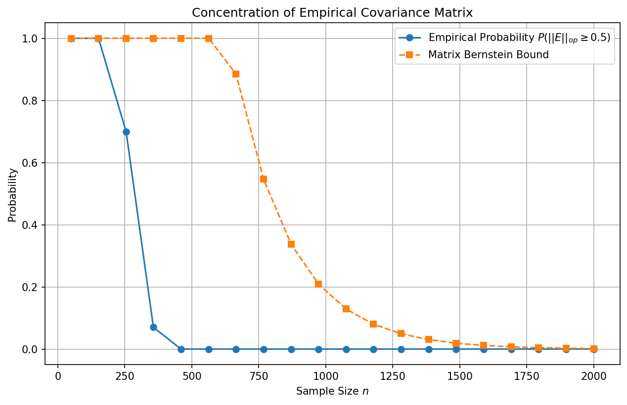
Demo 1: Matrix Bernstein and Empirical Covariance
This Python code using NumPy demonstrates the Matrix Bernstein bound in action by simulating the empirical covariance convergence of bounded random vectors.
import matplotlib
matplotlib.use('Agg')
import numpy as np
import matplotlib.pyplot as plt

def matrix_bernstein_covariance_demo():
    """
    Demonstrates Matrix Bernstein inequality for empirical covariance estimation.
    We plot the empirical spectral norm error against the theoretical bound.
    """
    np.random.seed(42)
    d = 20        # Dimension
    B = d         # Bound on squared norm
    num_trials = 100
    n_values = np.linspace(50, 2000, 20).astype(int)

    # True covariance is Identity for simplicity
    Sigma = np.eye(d)

    empirical_errors = []
    theoretical_errors = []

    t_fixed = 0.5 # We look at the probability of exceeding t=0.5

    for n in n_values:
        violations = 0
        for _ in range(num_trials):
            # Generate bounded vectors on a sphere of radius sqrt(B)
            # This ensures ||y||^2 <= B
            Y = np.random.randn(n, d)
            norms = np.linalg.norm(Y, axis=1, keepdims=True)
            Y = Y / norms * np.sqrt(d) # norm is exactly sqrt(d) = sqrt(B)

            # Empirical covariance
            Sigma_hat = (Y.T @ Y) / n

            # Operator norm error
            error = np.linalg.norm(Sigma_hat - Sigma, ord=2)
            if error >= t_fixed:
                violations += 1

        prob_empirical = violations / num_trials
        empirical_errors.append(prob_empirical)

        # Theoretical Matrix Bernstein Bound
        R = 2 * B / n
        sigma_sq = B * 1.0 / n # ||Sigma||_op = 1
        bound = d * np.exp(- (t_fixed**2 / 2) / (sigma_sq + R * t_fixed / 3))
        theoretical_errors.append(min(bound, 1.0)) # Probability <= 1

    plt.figure(figsize=(10, 6))
    plt.plot(n_values, empirical_errors, 'o-', label=r'Empirical Probability $P(||E||_{op} \geq 0.5)$')
    plt.plot(n_values, theoretical_errors, 's--', label='Matrix Bernstein Bound')
    plt.xlabel('Sample Size $n$')
    plt.ylabel('Probability')
    plt.title('Concentration of Empirical Covariance Matrix')
    plt.legend()
    plt.grid(True)
    plt.savefig('figures/03-1-demo1.png', dpi=150, bbox_inches='tight')
    plt.close()

matrix_bernstein_covariance_demo()
Demo 2: Empirical Wasserstein Distance via Sinkhorn Iterations
This PyTorch code demonstrates how to calculate the empirical Wasserstein distance using the Sinkhorn-Knopp algorithm, which regularizes the optimal transport problem with entropy, bridging the gap between metric distances and entropy exactly as discussed in the theory.
import torch

def sinkhorn_wasserstein(x, y, epsilon=0.01, iters=200):
    """
    Computes the entropically regularized 2-Wasserstein distance
    between two empirical distributions x and y using Sinkhorn iterations.

    Args:
        x: Tensor of shape (N, D) representing samples from mu
        y: Tensor of shape (M, D) representing samples from nu
        epsilon: Entropy regularization parameter
        iters: Number of Sinkhorn iterations
    """
    N = x.shape[0]
    M = y.shape[0]

    # Cost matrix: squared Euclidean distance
    # x: (N, 1, D), y: (1, M, D) -> C: (N, M)
    C = torch.sum((x.unsqueeze(1) - y.unsqueeze(0)) ** 2, dim=-1)

    # Gibbs kernel
    K = torch.exp(-C / epsilon)

    # Uniform marginals
    u = torch.ones(N, dtype=torch.float32) / N
    v = torch.ones(M, dtype=torch.float32) / M

    # Sinkhorn iterations
    for _ in range(iters):
        # Update u
        u = (1.0 / N) / (K @ v + 1e-8)
        # Update v
        v = (1.0 / M) / (K.T @ u + 1e-8)

    # Optimal transport plan
    P = torch.diag(u) @ K @ torch.diag(v)

    # Expected cost under the transport plan
    wasserstein_dist = torch.sum(P * C)

    return torch.sqrt(wasserstein_dist) # Return W_2, not W_2^2

def test_sinkhorn():
    # Generate two 2D Gaussian distributions
    torch.manual_seed(42)
    dist1 = torch.randn(200, 2)
    # Shifted distribution
    dist2 = torch.randn(200, 2) + torch.tensor([3.0, 3.0])

    w_dist = sinkhorn_wasserstein(dist1, dist2, epsilon=5.0, iters=200)
    print(f"Computed 2-Wasserstein distance: {w_dist.item():.4f}")

    # Theoretical W2 distance between N(0, I) and N(mu, I) is ||mu||_2
    theoretical_w2 = torch.norm(torch.tensor([3.0, 3.0]))
    print(f"Theoretical W2 distance: {theoretical_w2.item():.4f}")

# Execute test
test_sinkhorn()
These techniques heavily underscore the transition in modern learning theory from classical scalar bounds to rich, geometric, and matrix-valued analytical frameworks.