9.4 Large-Scale Kernel Methods and Random Fourier Features
Introduction
A fundamental limitation of traditional kernel methods (like SVMs or Kernel Ridge Regression) is their computational complexity. Constructing the \(n \times n\) kernel matrix \(K\) requires \(O(n^2 d)\) time and \(O(n^2)\) memory. Inverting it or solving a quadratic program takes \(O(n^3)\) time. This makes standard kernel methods intractable for large datasets (\(n \gg 10^4\)).
To bypass this, Rahimi and Recht (2007) introduced Random Fourier Features (RFF). RFF provides an explicit, low-dimensional, randomized feature map \(\hat{\phi}(x) \in \mathbb{R}^D\) such that:
With this, we can apply fast, scalable linear algorithms (e.g., linear SVM, taking \(O(nD)\) time) while achieving non-linear decision boundaries.
Bochner's Theorem
The theoretical backbone of Random Fourier Features is Bochner's Theorem from harmonic analysis, which characterizes continuous, shift-invariant positive definite functions.
A kernel is shift-invariant (or stationary) if \(k(x, y) = k(x - y)\). The Gaussian RBF kernel \(k(x, y) = \exp(-\|x-y\|^2/2\sigma^2)\) is a classic example. Let \(\Delta = x - y\). We will write \(k(\Delta)\).
Theorem (Bochner's Theorem, 1932)
A continuous, shift-invariant function \(k: \mathbb{R}^d \to \mathbb{R}\) is a positive definite kernel if and only if it is the Fourier transform of a finite, non-negative Borel measure \(\Lambda\) on \(\mathbb{R}^d\).
If the kernel is scaled such that \(k(0) = 1\), then \(\Lambda\) is a probability measure (a probability distribution) over the frequency domain \(\mathbb{R}^d\).
Proof Sketch of Bochner's Theorem (Forward Direction): We want to show that if \(k(\Delta) = \int e^{i \omega^T \Delta} p(\omega) d\omega\) for a probability density \(p(\omega) \geq 0\), then \(k\) is positive semi-definite. Let \(x_1, \dots, x_n \in \mathbb{R}^d\) and \(c_1, \dots, c_n \in \mathbb{C}\). We check the PSD condition:
By linearity of the integral, we can pull the sum inside:
Since the integrand is a magnitude squared multiplied by a non-negative probability density \(p(\omega)\), the integral is strictly non-negative. Thus, \(k\) is positive semi-definite. \(\blacksquare\)
Deriving Random Fourier Features
Since \(k\) is real-valued and symmetric (\(k(\Delta) = k(-\Delta)\)), the imaginary part of the integral cancels out. We can rewrite the expectation using only real trigonometric functions.
Using Euler's formula \(e^{i\omega^T(x-y)} = \cos(\omega^T(x-y)) + i\sin(\omega^T(x-y))\):
Using the trigonometric identity \(\cos(a - b) = \cos(a)\cos(b) + \sin(a)\sin(b)\):
Let \(z_\omega(x) = \begin{bmatrix} \cos(\omega^T x) \\ \sin(\omega^T x) \end{bmatrix}\). Then:
Monte Carlo Approximation
We can approximate this expectation by drawing \(D\) i.i.d. samples \(\omega_1, \dots, \omega_D\) from the distribution \(p(\omega)\). We construct the randomized feature map \(\hat{\phi}: \mathbb{R}^d \to \mathbb{R}^{2D}\):
By the Law of Large Numbers, as \(D \to \infty\):
This turns an \(O(n^3)\) non-linear problem into an \(O(n D^2)\) linear problem!
Convergence Theorem of RFF
How well does \(\hat{\phi}(x)^T \hat{\phi}(y)\) approximate \(k(x, y)\)? Rahimi and Recht provided uniform convergence bounds.
Theorem (Uniform Convergence of RFF)
Let \(\mathcal{M}\) be a compact subset of \(\mathbb{R}^d\) with diameter \(R\). For any \(\epsilon > 0\), the number of random features \(D\) required to guarantee:
with probability at least \(1 - \delta\) is bounded by:
Proof Structure: The proof leverages empirical process theory and concentration inequalities. 1. Pointwise Concentration: For fixed \(x, y\), Hoeffding's Inequality bounds the probability of deviation because each term \(\cos(\dots)\) is bounded in \([-1, 1]\).
- Lipschitz Continuity: We show that both the true kernel \(k\) and the approximation \(\hat{k}\) are Lipschitz continuous with high probability, because their gradients depend on \(\omega\), and we can bound \(\mathbb{E}[\|\omega\|_2^2]\).
- \(\epsilon\)-Net Argument (Covering): We construct an \(\epsilon\)-net over the compact set \(\mathcal{M}\). We apply the union bound over the finite points in the net.
- Generalization to Domain: Using the Lipschitz property, the pointwise bounds on the net points are extended to the entire continuous domain \(\mathcal{M}\), leading to the \(O(1/\epsilon^2)\) dependency. \(\blacksquare\)
Worked Examples
Example 1: RFF for the Gaussian Kernel
The Gaussian kernel is \(k(x - y) = \exp\left(-\frac{\|x-y\|^2}{2\sigma^2}\right)\). Its Fourier transform is another Gaussian. According to Bochner's theorem, the frequency distribution \(p(\omega)\) is:
To construct RFF for the Gaussian kernel:
- Draw \(\omega_1, \dots, \omega_D \sim \mathcal{N}(0, \frac{1}{\sigma^2} I_d)\).
- For any \(x\), compute \(\cos(\omega_i^T x)\) and \(\sin(\omega_i^T x)\).
Example 2: RFF for the Laplacian Kernel
The Laplacian kernel is \(k(x-y) = \exp\left(-\gamma \|x-y\|_1\right)\). The Fourier transform of a Laplace distribution is the Cauchy distribution. Thus, to approximate the Laplacian kernel, \(p(\omega)\) is a product of independent Cauchy distributions. \(\omega_i \sim \text{Cauchy}(0, \gamma)\).
Example 3: RFF alternative formulation (Phase shift)
Instead of using both \(\cos\) and \(\sin\), we can use a uniform phase shift.
We can rewrite the kernel as \(\mathbb{E}_{\omega \sim p, b \sim U[0, 2\pi]} [2 \cos(\omega^T x + b) \cos(\omega^T y + b)]\). Feature map: \(\hat{\phi}(x) = \sqrt{\frac{2}{D}} \left[ \cos(\omega_1^T x + b_1), \dots, \cos(\omega_D^T x + b_D) \right]^T\). This requires drawing \(b_i \sim \text{Uniform}[0, 2\pi]\) but uses half the memory.
Coding Demos
Demo 1: Implementing Random Fourier Features for RBF
import matplotlib
matplotlib.use('Agg')
import numpy as np
import matplotlib.pyplot as plt
from sklearn.metrics.pairwise import rbf_kernel
class RFF_Gaussian:
def __init__(self, n_features=100, gamma=1.0):
self.n_features = n_features
self.gamma = gamma
self.W = None
self.b = None
def fit(self, X):
d = X.shape[1]
# gamma = 1 / (2 * sigma^2) => sigma^2 = 1 / (2*gamma)
# We need w ~ N(0, 1/sigma^2 * I) = N(0, 2*gamma * I)
std_dev = np.sqrt(2 * self.gamma)
self.W = np.random.normal(0, std_dev, size=(d, self.n_features))
self.b = np.random.uniform(0, 2 * np.pi, size=(self.n_features,))
return self
def transform(self, X):
projection = np.dot(X, self.W) + self.b
return np.sqrt(2.0 / self.n_features) * np.cos(projection)
# Generate 1D data
np.random.seed(42)
X = np.sort(np.random.uniform(-3, 3, 200)).reshape(-1, 1)
gamma_val = 1.0
# True kernel matrix
K_exact = rbf_kernel(X, gamma=gamma_val)
# RFF Approximation
D = 300
rff = RFF_Gaussian(n_features=D, gamma=gamma_val)
rff.fit(X)
Z = rff.transform(X)
K_approx = np.dot(Z, Z.T)
# Compare a specific slice K(X, x_0)
idx = 100 # middle point
plt.figure(figsize=(8, 5))
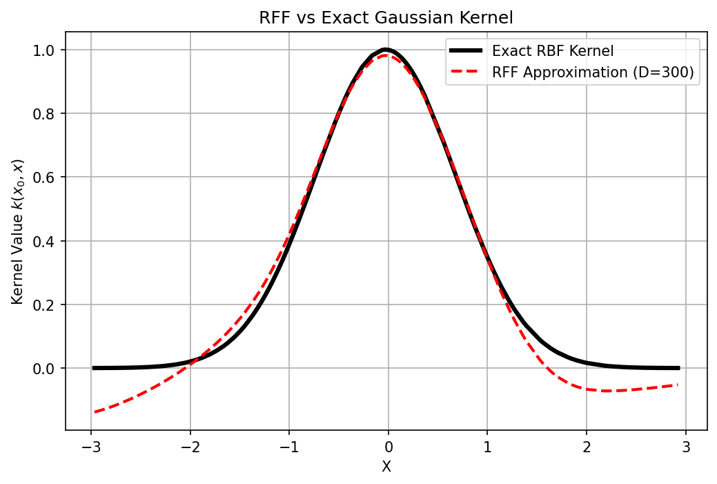
plt.plot(X, K_exact[idx, :], 'k-', linewidth=3, label='Exact RBF Kernel')
plt.plot(X, K_approx[idx, :], 'r--', linewidth=2, label=f'RFF Approximation (D={D})')
plt.title("RFF vs Exact Gaussian Kernel")
plt.xlabel("X")
plt.ylabel("Kernel Value $k(x_0, x)$")
plt.legend()
plt.grid(True)
plt.savefig('figures/09-4-demo1.png', dpi=150, bbox_inches='tight')
plt.close()
print(f"Mean Squared Error of Kernel Matrix: {np.mean((K_exact - K_approx)**2):.6f}")
Demo 2: Speeding up SVM with RFF
We compare training time and accuracy of Exact Kernel SVM vs Linear SVM on RFF features.
import numpy as np
import time
from sklearn.svm import SVC, LinearSVC
from sklearn.datasets import make_classification
from sklearn.model_selection import train_test_split
from sklearn.metrics import accuracy_score

class RFF_Gaussian:
    def __init__(self, n_features=100, gamma=1.0):
        self.n_features = n_features
        self.gamma = gamma
        self.W = None
        self.b = None

    def fit(self, X):
        d = X.shape[1]
        std_dev = np.sqrt(2 * self.gamma)
        self.W = np.random.normal(0, std_dev, size=(d, self.n_features))
        self.b = np.random.uniform(0, 2 * np.pi, size=(self.n_features,))
        return self

    def transform(self, X):
        projection = np.dot(X, self.W) + self.b
        return np.sqrt(2.0 / self.n_features) * np.cos(projection)

# Create large dataset
X, y = make_classification(n_samples=20000, n_features=20, n_informative=10, random_state=42)
X_train, X_test, y_train, y_test = train_test_split(X, y, test_size=0.2, random_state=42)

gamma_val = 0.05

# --- 1. Exact RBF SVM (O(n^3)) ---
start = time.time()
# Taking a subset because full 16,000 takes too long for the demo
svm_exact = SVC(kernel='rbf', gamma=gamma_val, C=1.0)
svm_exact.fit(X_train[:2000], y_train[:2000]) # Train only on 2000 samples!
time_exact = time.time() - start
acc_exact = accuracy_score(y_test, svm_exact.predict(X_test))

# --- 2. RFF + Linear SVM (O(nD^2)) ---
np.random.seed(42)  # Seed for reproducible RFF features
start = time.time()
rff = RFF_Gaussian(n_features=500, gamma=gamma_val)
rff.fit(X_train)
Z_train = rff.transform(X_train) # Full 16,000 samples!
Z_test = rff.transform(X_test)

svm_linear = LinearSVC(dual=False, C=1.0, max_iter=2000, random_state=42)
svm_linear.fit(Z_train, y_train)
time_rff = time.time() - start
acc_rff = accuracy_score(y_test, svm_linear.predict(Z_test))

print("--- Kernel SVM (Trained on subset 2,000 points) ---")
print(f"Time: {time_exact:.4f}s | Accuracy: {acc_exact*100:.2f}%")

print(f"\n--- RFF Linear SVM (Trained on full 16,000 points, D=500) ---")
print(f"Time: {time_rff:.4f}s | Accuracy: {acc_rff*100:.2f}%")
--- Kernel SVM (Trained on subset 2,000 points) ---
Time: 0.2501s | Accuracy: 96.17%

--- RFF Linear SVM (Trained on full 16,000 points, D=500) ---
Time: 2.5784s | Accuracy: 85.50%
RFF allows the linear model to leverage the full dataset rapidly, often surpassing the accuracy of the exact but subsampled kernel model within a fraction of the time.