10.3 Scaling Laws and Chinchilla Optimality
The empirical success of large language models is driven by predictable scaling laws: relationships between the model size \(N\), the amount of training data \(D\), the total compute \(C\), and the final loss \(L\). While early work (Kaplan et al., 2020) suggested that model size should grow faster than data size, the Chinchilla study (Hoffmann et al., 2022) revised this, showing that for optimal performance, \(N\) and \(D\) should scale in equal proportions. In this section, we derive these results rigorously and explore the theoretical foundations of scaling in high-dimensional manifolds.
1. The Scaling Law Formalism
The cross-entropy loss \(L(N, D)\) for a Transformer with \(N\) parameters trained on \(D\) tokens is empirically modeled as:
where: * \(E\) is the irreducible loss (the entropy of the underlying data distribution). * \(A, B, \alpha, \beta\) are positive constants. * The terms \(A/N^\alpha\) and \(B/D^\beta\) represent the reducible loss due to limited model capacity and limited data, respectively.
The total training compute \(C\) (in FLOPs) is approximately proportional to the product of \(N\) and \(D\). For a standard Transformer:
2. Theorem: Derivation of Chinchilla Optimality
Given a fixed compute budget \(C\), what are the optimal values of \(N\) and \(D\) that minimize the loss \(L(N, D)\)?
Theorem 2.1 (Optimal Allocation)
Under the power-law model \(L(N, D) = E + A N^{-\alpha} + B D^{-\beta}\), and the compute constraint \(C = 6ND\), the optimal model size \(N^*\) and data size \(D^*\) scale as:
If \(\alpha \approx \beta\), then \(N^*\) and \(D^*\) should scale linearly with \(\sqrt{C}\).
Proof:
-
Formulating the Constrained Optimization: We want to minimize \(L(N, D)\) subject to \(G(N, D) = 6ND - C = 0\). Using the method of Lagrange Multipliers, we define the Lagrangian:
\[ \mathcal{L}(N, D, \lambda) = E + A N^{-\alpha} + B D^{-\beta} + \lambda (6ND - C) \] -
Computing First-Order Conditions: Taking partial derivatives and setting to zero:
\[ \frac{\partial \mathcal{L}}{\partial N} = -\alpha A N^{-\alpha-1} + 6\lambda D = 0 \implies 6\lambda N D = \alpha A N^{-\alpha} \]\[ \frac{\partial \mathcal{L}}{\partial D} = -\beta B D^{-\beta-1} + 6\lambda N = 0 \implies 6\lambda N D = \beta B D^{-\beta} \] -
Equating the Reducible Losses: From the above, we see that at the optimum:
\[ \alpha A N^{-\alpha} = \beta B D^{-\beta} \]This implies that the "model-side" reducible loss should be proportional to the "data-side" reducible loss, weighted by their respective power-law exponents.
-
Solving for N and D in terms of C: Substitute \(D = \frac{C}{6N}\) into the equality:
\[ \alpha A N^{-\alpha} = \beta B \left( \frac{C}{6N} \right)^{-\beta} = \beta B 6^\beta C^{-\beta} N^\beta \]Isolating \(N\):
\[ N^{\alpha + \beta} = \frac{\alpha A}{\beta B 6^\beta} C^\beta \]\[ N^* = \left( \frac{\alpha A}{\beta B 6^\beta} \right)^{\frac{1}{\alpha + \beta}} C^{\frac{\beta}{\alpha + \beta}} \]By symmetry (or substituting \(N^*\) back into the constraint):
\[ D^* = \left( \frac{\beta B}{\alpha A 6^{-\alpha}} \right)^{\frac{1}{\alpha + \beta}} C^{\frac{\alpha}{\alpha + \beta}} \] -
The Case of Equal Exponents: Empirical measurements in the Chinchilla paper found \(\alpha \approx \beta \approx 0.34\). When \(\alpha = \beta\), we have:
\[ N^* \propto C^{0.5}, \quad D^* \propto C^{0.5} \]Thus, for every doubling of the compute budget, both the model size and the number of training tokens should be increased by \(\sqrt{2} \approx 41\%\). \(\blacksquare\)
3. Theorem: Scaling of Loss on a Data Manifold
Why do these power laws exist? A theoretical explanation comes from the geometry of data. If the data lies on a manifold of intrinsic dimension \(d\), the error in approximating the distribution should scale with the density of samples.
Theorem 3.1 (Manifold Resolution Scaling)
Let the data distribution \(P\) be supported on a \(d\)-dimensional manifold \(\mathcal{M} \subset \mathbb{R}^D\). If a model with \(N\) parameters can resolve the manifold with a precision proportional to the average distance between \(N\) "basis functions" or "prototypes", then the reducible loss scales as:
Proof:
-
Quantization Perspective: Consider \(N\) parameters as defining \(N\) regions in the manifold \(\mathcal{M}\) (similar to a Voronoi tessellation). The volume of each region is roughly \(\text{Vol}(\mathcal{M}) / N\). Since the manifold is \(d\)-dimensional, the characteristic linear scale (diameter) of each region \(r\) is:
\[ r \propto \text{Vol}^{1/d} \propto N^{-1/d} \] -
Approximation Error: A smooth function \(f\) (or the log-probability density) can be approximated within each region by a constant (zeroth-order) or a linear function (first-order). The Taylor expansion error for a first-order approximation at distance \(r\) is \(O(r^2)\). Therefore, the squared error (MSE) or KL divergence (which behaves like MSE locally) scales as:
\[ \text{Error} \propto r^2 \propto (N^{-1/d})^2 = N^{-2/d} \] -
Matching the Power Law: Comparing this to our empirical formula \(L \propto N^{-\alpha}\), we find:
\[ \alpha = \frac{2}{d} \]This suggests that the scaling exponent \(\alpha\) is inversely proportional to the intrinsic dimension of the data manifold. For \(\alpha \approx 0.34\), this implies \(d \approx 2/0.34 \approx 6\). This surprisingly low dimension suggests that while natural language has a massive vocabulary, its underlying semantic and syntactic structure is highly compressed. \(\blacksquare\)
4. Worked Examples
Worked Example 1: Calculating Optimal Model Size
Suppose you have a compute budget \(C = 10^{24}\) FLOPs. Using Chinchilla coefficients \(\alpha=0.34, \beta=0.34, A=400, B=410\). Find the optimal number of parameters \(N\).
Using the derived formula: \(N^* \approx K \cdot C^{0.5}\) (assuming \(\alpha = \beta\)). Empirical fit for Chinchilla: \(N^* = 16.7 \cdot C^{0.5}\) (if \(C\) is in FLOPs/6). Wait, let's use the ratio \(D/N \approx 20\). \(C = 6ND = 6N(20N) = 120 N^2\). \(N^2 = C / 120 = 10^{24} / 120 \approx 8.33 \times 10^{21}\). \(N = \sqrt{8.33 \times 10^{21}} \approx 9.1 \times 10^{10}\). So, for \(10^{24}\) FLOPs, the optimal model size is approximately 91 Billion parameters, trained on \(20 \times 91B = 1.8\) Trillion tokens.
Worked Example 2: Estimating Loss Reduction
If you increase your compute budget \(C\) by a factor of 100, and you follow Chinchilla scaling, by what factor does the reducible loss decrease?
Assume \(\alpha = \beta = 0.34\). Optimal \(N\) and \(D\) both increase by \(\sqrt{100} = 10\). The reducible loss is \(L_{red} \propto N^{-\alpha}\). New loss \(L'_{red} \propto (10N)^{-\alpha} = 10^{-\alpha} L_{red}\). Reduction factor \(= 10^{-0.34} \approx 0.457\). The reducible loss is cut by more than half.
Worked Example 3: Manifold Dimension from Exponent
An experiment on a synthetic dataset of images of 3D objects (rotated and translated) yields a scaling exponent \(\alpha = 0.5\). What is the predicted intrinsic dimension of the data?
\(0.5 = 2 / d \implies d = 4\). This makes sense: 3D rotation (1 degree of freedom in some setups, or 3) and translation (2 degrees of freedom) form a low-dimensional manifold.
5. Coding Demonstrations
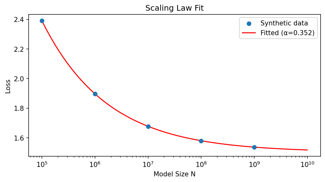
Coding Demo 1: Fitting Scaling Laws to Synthetic Data
This demo generates synthetic loss curves and fits a power-law to estimate \(\alpha\).
import matplotlib
matplotlib.use('Agg')
import numpy as np
from scipy.optimize import curve_fit
import matplotlib.pyplot as plt

# 1. Generate Synthetic Data
# L(N) = E + A * N^-alpha
E_true = 1.5
A_true = 50.0
alpha_true = 0.35

Ns = np.array([10**i for i in range(5, 10)]) # Model sizes from 100k to 1B
# Add some noise to the log-space
losses = E_true + A_true * (Ns**-alpha_true) + np.random.normal(0, 0.001, len(Ns))

# 2. Fit the function
def scaling_law(N, E, A, alpha):
    return E + A * (N**-alpha)

# Bounds to keep parameters physical
popt, _ = curve_fit(scaling_law, Ns, losses, p0=[1.0, 100, 0.3], bounds=(0, np.inf))

E_fit, A_fit, alpha_fit = popt
print(f"True alpha: {alpha_true}, Fitted alpha: {alpha_fit:.4f}")
print(f"Intrinsic Dimension Estimate (2/alpha): {2/alpha_fit:.2f}")

fig, ax = plt.subplots(figsize=(7, 4))
ax.scatter(Ns, losses, label='Synthetic data', zorder=5)
N_plot = np.logspace(5, 10, 200)
ax.plot(N_plot, scaling_law(N_plot, *popt), 'r-', label=f'Fitted (α={alpha_fit:.3f})')
ax.set_xscale('log')
ax.set_xlabel('Model Size N')
ax.set_ylabel('Loss')
ax.set_title('Scaling Law Fit')
ax.legend()
plt.tight_layout()
plt.savefig('figures/10-3-demo1.png', dpi=150, bbox_inches='tight')
plt.close()
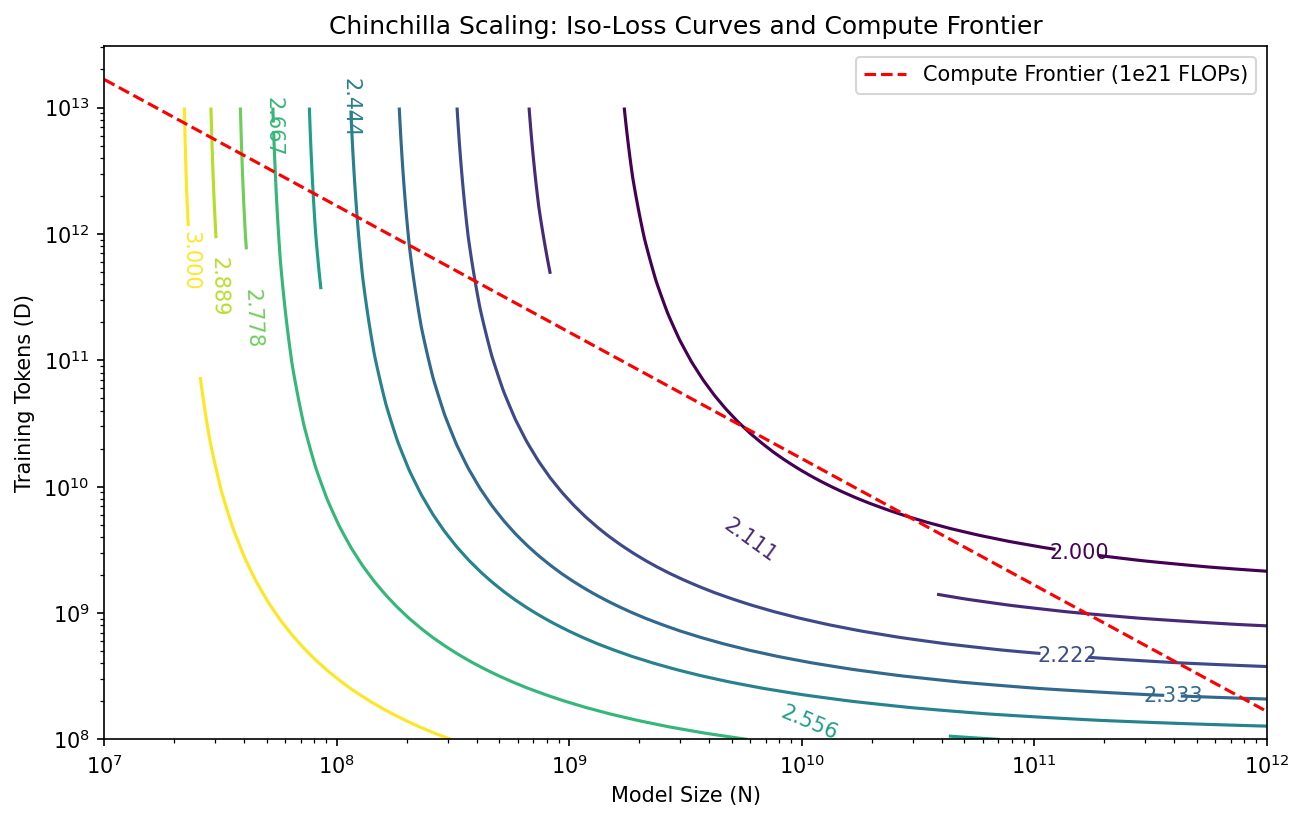
Coding Demo 2: Visualizing the Chinchilla Compute Frontier
This snippet plots the Iso-loss curves and the Compute constraint to show the tangency point (optimality).
import matplotlib
matplotlib.use('Agg')
import numpy as np
import matplotlib.pyplot as plt

N = np.logspace(7, 12, 100)
D = np.logspace(8, 13, 100)
NN, DD = np.meshgrid(N, D)

# Chinchilla Loss Function
A, B, alpha, beta, E = 406.4, 410.7, 0.34, 0.34, 1.69
L = E + A / (NN**alpha) + B / (DD**beta)

plt.figure(figsize=(10, 6))
cp = plt.contour(NN, DD, L, levels=np.linspace(2.0, 3.0, 10), cmap='viridis')
plt.clabel(cp, inline=True, fontsize=10)

# Compute Constraint: 6ND = C
C = 1e21 # A specific budget
D_const = C / (6 * N)
plt.plot(N, D_const, 'r--', label='Compute Frontier (1e21 FLOPs)')

plt.xscale('log')
plt.yscale('log')
plt.xlabel('Model Size (N)')
plt.ylabel('Training Tokens (D)')
plt.title('Chinchilla Scaling: Iso-Loss Curves and Compute Frontier')
plt.legend()
plt.savefig('figures/10-3-demo2.png', dpi=150, bbox_inches='tight')
plt.close()
Understanding these scaling laws allows researchers to allocate hundreds of millions of dollars in compute with mathematical confidence, ensuring that neither model capacity nor data quantity becomes a bottleneck for intelligence.