9.3 Mercer's Theorem and Spectral Theory of Kernels
Introduction
While the Moore-Aronszajn Theorem constructs the RKHS via completion of kernel linear combinations, Mercer's Theorem provides a profoundly different perspective. It approaches kernels from the viewpoint of integral operators and spectral theory. By decomposing a kernel into its eigenfunctions, Mercer's Theorem gives us an explicit orthogonal basis for the RKHS, linking kernel methods to functional analysis and Fourier theory.
This perspective is critical for understanding the capacity of kernel machines, the decay of eigenvalues (spectral decay), and generalization bounds.
Integral Operators and Mercer's Theorem
Let \(\mathcal{X} \subset \mathbb{R}^d\) be a compact metric space, and let \(\mu\) be a finite Borel measure on \(\mathcal{X}\) (such as the probability distribution of the data) strictly positive on open sets.
Let \(k \in L_\infty(\mathcal{X} \times \mathcal{X})\) be a symmetric positive semi-definite continuous kernel.
We can define an integral operator \(T_k : L_2(\mathcal{X}, \mu) \to L_2(\mathcal{X}, \mu)\) by:
Because \(k\) is continuous and \(\mathcal{X}\) is compact, \(T_k\) is a compact operator, and because \(k\) is symmetric, \(T_k\) is self-adjoint. Because \(k\) is PSD, \(T_k\) is a positive operator:
By the Spectral Theorem for compact self-adjoint operators, \(T_k\) has an at most countable set of non-negative eigenvalues \(\lambda_1 \geq \lambda_2 \geq \dots \geq 0\) and a corresponding set of orthogonal eigenfunctions \(\{e_n\}\) in \(L_2(\mathcal{X}, \mu)\) such that:
Mercer's Theorem (1909)
Theorem (Mercer's Theorem)
If \(k(x, y)\) is a continuous, symmetric, positive semi-definite kernel on a compact metric space \(\mathcal{X}\), then it can be expanded in an absolutely and uniformly convergent series:
where \(\lambda_n > 0\) are the strictly positive eigenvalues of the integral operator \(T_k\), and \(e_n\) are the corresponding continuous, \(L_2(\mu)\)-orthonormal eigenfunctions.
Proof Sketch: A full proof of Mercer's theorem requires deep functional analysis (specifically Dini's theorem and Mercer's original work). We outline the crucial structural steps:
-
Existence of Eigendecomposition: Since \(T_k\) is compact and self-adjoint, the Hilbert-Schmidt theorem guarantees an orthonormal basis of eigenfunctions \(\{e_n\}\) for \(L_2(\mathcal{X}, \mu)\).
-
Continuity of Eigenfunctions: For any \(e_n\) with \(\lambda_n > 0\), we have \(e_n(x) = \frac{1}{\lambda_n} \int k(x, y) e_n(y) d\mu(y)\). Since \(k(x, y)\) is continuous in \(x\) and uniformly bounded, the integral is continuous in \(x\). Thus, \(e_n\) (which are originally defined almost everywhere in \(L_2\)) have continuous representatives.
-
Positivity: Because \(k\) is PSD, \(\langle e_n, T_k e_n \rangle \geq 0 \implies \lambda_n \geq 0\).
-
Uniform Convergence (The Core of Mercer's Theorem): By defining \(k_N(x, y) = k(x, y) - \sum_{n=1}^N \lambda_n e_n(x) e_n(y)\), it can be shown that \(k_N\) is still a PSD kernel. Therefore, its diagonal elements are non-negative:
$$ k(x, x) - \sum_{n=1}^N \lambda_n e_n(x)^2 \geq 0 \implies \sum_{n=1}^N \lambda_n e_n(x)^2 \leq k(x, x) $$
Since \(k(x,x)\) is bounded (continuous on a compact set), the series of positive continuous functions \(\sum \lambda_n e_n(x)^2\) converges monotonically. By Dini's Theorem, pointwise convergence of a monotonic sequence of continuous functions to a continuous function on a compact set implies uniform convergence. From Cauchy-Schwarz, uniform convergence of the diagonal implies uniform convergence of the off-diagonal \(k(x, y)\).
\(\blacksquare\)
RKHS in the View of Mercer's Theorem
Using Mercer's theorem, we can explicitly define the RKHS \(\mathcal{H}\) associated with \(k\). Consider the set of functions:
The RKHS inner product is defined as:
where \(f = \sum a_n e_n\) and \(g = \sum b_n e_n\).
Let's verify the reproducing property. Let \(f \in \mathcal{H}\). Let's take the inner product with \(k(\cdot, x)\). By Mercer's Theorem, \(k(\cdot, x) = \sum \lambda_n e_n(x) e_n(\cdot)\). The sequence of coefficients for \(k_x\) is \(b_n = \lambda_n e_n(x)\).
This shows that the RKHS norm strongly penalizes functions that project heavily onto eigenfunctions with small eigenvalues \(\lambda_n\).
Spectral Decay and Function Smoothness
The rate at which the eigenvalues \(\lambda_n \to 0\) dictates the capacity of the RKHS. If \(\lambda_n\) decays rapidly (e.g., exponentially), the RKHS contains only very smooth functions. If it decays slowly (e.g., polynomially), the RKHS contains rougher functions.
Theorem (Spectral Decay of Gaussian Kernel)
For the Gaussian RBF kernel \(k(x, y) = \exp(-\frac{1}{2\sigma^2}\|x-y\|^2)\) and a Gaussian data measure \(\mu\), the eigenfunctions are given by Hermite polynomials, and the eigenvalues decay geometrically (exponentially): \(\lambda_n = O(c^n)\) for some \(0 < c < 1\).
Proof Outline: 1. In 1D, let \(p(x) \propto \exp(-x^2/2\sigma_x^2)\). 2. We seek solutions to \(\int \exp(-\frac{(x-y)^2}{2\sigma^2}) \exp(-\frac{y^2}{2\sigma_x^2}) e_n(y) dy = \lambda_n e_n(x)\). 3. This is an instance of the Gaussian integral transformation. The solutions \(e_n(x)\) are Hermite polynomials multiplied by a Gaussian envelope. 4. The corresponding eigenvalues follow the exact formula \(\lambda_n \propto (1 + 2\frac{\sigma_x^2}{\sigma^2} + \sqrt{1 + 4\frac{\sigma_x^2}{\sigma^2}})^{-n}\), which exhibits an exponential decay \(\lambda_n = c^n\) where \(c < 1\).
Because \(\lambda_n\) drops so fast, for \(f = \sum a_n e_n\) to have a finite RKHS norm \(\sum \frac{a_n^2}{\lambda_n} < \infty\), the coefficients \(a_n\) of the high-frequency Hermite polynomials must decay even faster than \(\sqrt{\lambda_n}\). This forces \(f\) to be extremely smooth.
Worked Examples
Example 1: Eigenfunctions of the Linear Kernel
Let \(k(x, y) = x^T y\) on the unit sphere \(\mathcal{X} = S^{d-1}\) with uniform measure. The integral operator is \((T_k f)(x) = \int_{S^{d-1}} (x^T y) f(y) dy\). Notice that \(x^T y = \sum_{i=1}^d x_i y_i\). Let \(e_i(x) = x_i\). Then \((T_k e_i)(x) = \sum_{j} x_j \int y_j y_i dy\). By orthogonality of coordinates on the sphere, this is proportional to \(x_i\). Thus, the coordinate functions \(x_i\) are the eigenfunctions, and there are exactly \(d\) non-zero eigenvalues. The kernel has finite rank.
Example 2: The Sobolev Space equivalent RKHS
Consider the Laplace kernel \(k(x, y) = \exp(-\|x-y\|_1)\). Its eigenvalues decay polynomially: \(\lambda_n = O(n^{-2})\). This maps directly to the Sobolev space \(H^1\) of functions with square-integrable first derivatives. It allows for non-differentiable "kinks" in the functions, making it a "rougher" RKHS compared to the Gaussian kernel.
Example 3: Infinite Capacity
For the Gaussian kernel, since \(\lambda_n > 0\) for all \(n \in \mathbb{N}\), the feature space is infinite-dimensional. Because it contains basis functions of arbitrarily high frequencies (though heavily penalized), it acts as a universal approximator on compact sets.
Coding Demos
Demo 1: Empirical Spectral Decay of Kernels
We will compute the empirical eigenvalues of the Kernel matrix \(K\) scaled by \(1/n\) (which approximates the integral operator \(T_k\)) and observe the decay rates for RBF vs Laplace kernels.
import matplotlib
matplotlib.use('Agg')
import numpy as np
import matplotlib.pyplot as plt
from sklearn.metrics.pairwise import rbf_kernel, laplacian_kernel

# 1. Generate uniform data in [0, 1]^d
np.random.seed(42)
n_samples = 1000
X = np.random.rand(n_samples, 2)

# 2. Compute kernels
K_rbf = rbf_kernel(X, gamma=10.0)
K_lap = laplacian_kernel(X, gamma=10.0)

# 3. Compute eigenvalues (Hermitian/Symmetric matrix)
eigvals_rbf = np.linalg.eigvalsh(K_rbf / n_samples)
eigvals_lap = np.linalg.eigvalsh(K_lap / n_samples)

# Sort in descending order
eigvals_rbf = np.sort(eigvals_rbf)[::-1]
eigvals_lap = np.sort(eigvals_lap)[::-1]

# 4. Plot
plt.figure(figsize=(10, 6))
plt.plot(eigvals_rbf[:100], label='RBF (Gaussian) Kernel', linewidth=2)
plt.plot(eigvals_lap[:100], label='Laplacian Kernel', linewidth=2)
plt.yscale('log')
plt.title("Empirical Spectral Decay of Kernels (First 100 Eigenvalues)")
plt.xlabel("Index $n$")
plt.ylabel(r"Eigenvalue $\lambda_n$ (Log Scale)")
plt.legend()
plt.grid(True)
plt.savefig('figures/09-3-demo1.png', dpi=150, bbox_inches='tight')
plt.close()
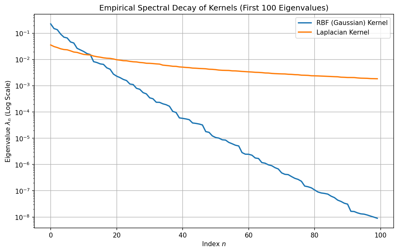 Observation: The RBF kernel eigenvalues plummet exponentially, reaching machine precision quickly, confirming it forms a very smooth RKHS. The Laplacian kernel eigenvalues decay linearly in log-space (polynomially), indicating higher capacity for rough functions.
Demo 2: Mercer Expansion Approximation (Nyström Method)
We can approximate a kernel matrix using a subset of points (landmarks) by relying on the eigenvectors of the sub-matrix. This is essentially empirical Mercer decomposition.
import numpy as np
from scipy.linalg import eigh
from sklearn.metrics.pairwise import rbf_kernel

def nystrom_approximation(X, n_components=50, gamma=1.0):
    n = X.shape[0]

    # Randomly select landmark points
    indices = np.random.permutation(n)[:n_components]
    X_landmarks = X[indices]

    # Compute K_MM (landmarks x landmarks)
    K_MM = rbf_kernel(X_landmarks, gamma=gamma)

    # Eigendecomposition of K_MM
    eigvals, eigvecs = eigh(K_MM)

    # Keep strictly positive eigvals
    mask = eigvals > 1e-10
    eigvals = eigvals[mask]
    eigvecs = eigvecs[:, mask]

    # Compute K_NM (all points x landmarks)
    K_NM = rbf_kernel(X, X_landmarks, gamma=gamma)

    # Approximate eigenfunctions for all X
    # e_n(x) \approx \frac{1}{\lambda_n} \sum K(x, x_m) v_{m,n}
    phi = K_NM @ (eigvecs / np.sqrt(eigvals))

    # Approximate K \approx \Phi \Phi^T
    return phi, eigvals

# Test approximation
np.random.seed(42)
n_samples = 800
X_full = np.random.randn(n_samples, 2)
K_exact = rbf_kernel(X_full, gamma=0.5)

phi, _ = nystrom_approximation(X_full, n_components=100, gamma=0.5)
K_approx = phi @ phi.T

error = np.linalg.norm(K_exact - K_approx, ord='fro') / np.linalg.norm(K_exact, ord='fro')
print(f"Relative Frobenius norm error with 100 landmarks (out of {n_samples}): {error*100:.2f}%")
This Nyström approximation is heavily used in large-scale kernel methods, relying directly on the existence of Mercer's eigendecomposition.