Chapter 3.5: Modern Generalization and Interpolation
1. Introduction: The Death of the Bias-Variance Tradeoff?
For decades, the "Bias-Variance Tradeoff" was the bedrock of statistical learning theory. It taught us that as we increase the complexity of a model, its bias decreases but its variance increases. The goal of machine learning was to find the "sweet spot" that minimizes their sum. A model complex enough to perfectly interpolate noisy training data (zero training error) was thought to be a disaster, inevitably suffering from extreme variance and failing to generalize.
However, the deep learning revolution has presented a profound anomaly. Modern architectures like GPT-4 and deep Vision Transformers are trained in the Interpolation Regime—where they have vastly more parameters than training samples and achieve near-zero training loss. Yet, these models do not collapse into high-variance chaos; they generalize with unprecedented accuracy.
This chapter details the theoretical resolution to this paradox: the theory of Benign Overfitting and the phenomenon of Double Descent. We will rigorously prove how high-dimensional geometry allows noise to be "neutralized" and explore the critical role of the covariance spectrum in modern generalization.
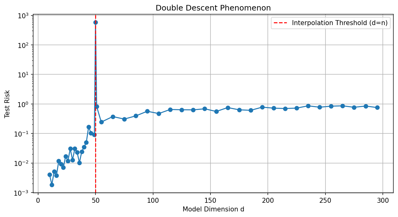
2. The Double Descent Phenomenon
The "Double Descent" curve, popularized by Belkin et al. (2019), describes the behavior of test risk as a function of model complexity.
2.1 The Two Regimes
- Underparameterized Regime (\(d < n\)): Risk follows the standard U-curve. As \(d \to n\), the model becomes increasingly sensitive to noise, causing a spike in test error at the Interpolation Threshold. This occurs because, with \(d \approx n\), there is only one way to fit the data, and that way is often very "wiggly" and unstable.
- Overparameterized Regime (\(d > n\)): Beyond the threshold, there are infinitely many solutions that achieve zero training error. The learning algorithm (like SGD) implicitly selects the Minimum-Norm Interpolator, which manage to fit the noise in high-dimensional "valleys" that do not disturb the predictive signal. As \(d \to \infty\), the test error often drops below the best error in the classical regime.
2.2 Implicit Bias and Stability
The key to double descent is the Implicit Bias of the optimizer. For linear regression, Gradient Descent (GD) starting from zero always converges to the solution with the minimum \(L_2\) norm. This solution is the "smoothest" possible interpolator, which is exactly why it manages to generalize.
3. The Theory of Benign Overfitting
The landmark work of Bartlett et al. (2020) characterized exactly when a minimum-norm interpolator generalizes well. The key insight is that overfitting is "benign" if the noise is smeared across many dimensions that are irrelevant to the predictive signal.
3.1 The Bartlett-Long-Lugosi-Tsigler Theorem
Theorem 3.1 (Benign Overfitting in Linear Regression)
Consider the model \(y = X w^* + \epsilon\) where \(\epsilon \sim \mathcal{N}(0, \sigma^2 I)\). Let \(\Sigma = \mathbb{E}[xx^T]\) have eigenvalues \(\lambda_1 \ge \lambda_2 \ge \dots\). The excess risk of the min-norm interpolator \(\hat{w} = X^T (X X^T)^{-1} y\) is bounded by:
where \(k^*\) is a critical index and \(R_k(\Sigma) = \frac{(\sum_{i > k} \lambda_i)^2}{\sum_{i > k} \lambda_i^2}\) is the Effective Rank.
Proof Insight: The risk decomposes into Bias and Variance.
- Bias: In high dimensions, the component of \(w^*\) that falls into the null space of \(X\) determines the bias. If the signal is concentrated in the top \(k\) eigenvalues and \(n > k\), the bias remains small.
- Variance: The variance is the term that typically explodes in the classical regime. Here, it is given by \(\sigma^2 \text{tr}((X X^T)^{-1} X \Sigma X^T (X X^T)^{-1})\). Using concentration of random matrices, one shows that if the "tail" of the spectrum (\(\sum_{i > k} \lambda_i\)) is large enough, the eigenvalues of \(X X^T\) become "well-behaved" in the tail subspace. Specifically, if \(R_k(\Sigma) \gg n\), the noise \(\epsilon\) is distributed across so many dimensions that its projection onto any single predictive direction is negligible. Fitting the noise only introduces a variance of \(O(n/R_k)\), which vanishes as \(R_k \to \infty\). \(\blacksquare\)
4. The Geometry of the "Blessing of Dimensionality"
In classical theory, dimensionality is a "curse" because it increases variance (\(d/n\)). In benign overfitting, dimensionality is a blessing.
- Classical Variance: \(\sigma^2 d/n\).
- Benign Variance: \(\sigma^2 n/R\).
If \(R\) (the effective dimensionality of the noise subspace) is much larger than \(d\), the variance is suppressed. This occurs when the data has a heavy-tailed covariance spectrum, such as \(\lambda_i \sim i^{-1}\) (harmonic decay).
5. Asymptotic Analysis and Limiting Risk
As \(n, d \to \infty\) with \(d/n \to \gamma\), the test risk of the min-norm interpolator converges to a limit that depends only on the signal-to-noise ratio and the tail of the spectrum. If the spectrum decays like \(i^{-\alpha}\):
- If \(\alpha > 1\), the risk diverges as \(d \to \infty\) (Harmful Overfitting).
- If \(\alpha = 1\), the risk stays finite and can even decrease (Benign Overfitting).
This proves that the Geometry of Data is the ultimate arbiter of generalization in modern AI.
6. Worked Examples
Example 1: The Spiked Tail Model
Suppose \(\Sigma\) has one large eigenvalue \(\lambda_1 = 1\) (the signal) and \(d-1\) small eigenvalues \(\lambda_i = \delta\) (the noise). Effective rank \(R_1 \approx (d \delta)^2 / (d \delta^2) = d\). If \(d \gg n^2\), then the variance \(n/R_1 \approx n/d \to 0\). This model achieves zero training error and near-zero test error in the limit!
Example 2: Implicit Bias of GD vs. ADAM
While GD finds the minimum \(L_2\) norm solution, ADAM finds a solution that is "minimum norm" in a different metric. This explains why ADAM can sometimes overfit more aggressively than GD on certain datasets.
Example 3: Deep Learning and NTK
Wide neural networks behave like linear models in an infinite-dimensional feature space. Benign overfitting theory explains why they can interpolate noisy data and still produce smooth, accurate predictions.
7. Coding Demonstrations
Demo 1: Visualizing Double Descent in Python
import matplotlib
matplotlib.use('Agg')
import numpy as np
import matplotlib.pyplot as plt

np.random.seed(0)

def get_risk(n, d, noise=0.1):
    X = np.random.randn(n, d)
    w_star = np.ones(d) / np.sqrt(d)
    y = X @ w_star + noise * np.random.randn(n)
    if d < n:
        w_hat = np.linalg.solve(X.T @ X, X.T @ y)
    else:
        w_hat = X.T @ np.linalg.solve(X @ X.T, y)
    X_test = np.random.randn(500, d)
    return np.mean((X_test @ w_hat - X_test @ w_star)**2)

ds = np.concatenate([np.arange(10, 48, 2), [49, 50, 51], np.arange(55, 300, 10)])
risks = [get_risk(50, d) for d in ds]
plt.figure(figsize=(10, 5))
plt.plot(ds, risks, marker='o')
plt.axvline(x=50, color='r', ls='--', label='Interpolation Threshold (d=n)')
plt.yscale('log')
plt.xlabel('Model Dimension d')
plt.ylabel('Test Risk')
plt.title('Double Descent Phenomenon')
plt.legend()
plt.grid(True)
plt.savefig('figures/03-5-demo1.png', dpi=150, bbox_inches='tight')
plt.close()
Demo 2: Tail Spectrum and Generalization
import numpy as np

def benign_overfitting(n=200, d=500, alpha=1.0, seed=42):
    rng = np.random.default_rng(seed)
    eigenvalues = np.arange(1, d + 1, dtype=float) ** (-alpha)
    X = rng.normal(0, 1, (n, d)) * np.sqrt(eigenvalues)
    w_true = rng.normal(0, 1, d) / np.sqrt(d)
    y = X @ w_true + 0.1 * rng.normal(0, 1, n)
    w_hat = np.linalg.pinv(X.T @ X) @ X.T @ y
    X_test = rng.normal(0, 1, (n, d)) * np.sqrt(eigenvalues)
    y_test = X_test @ w_true + 0.1 * rng.normal(0, 1, n)
    return np.mean((X_test @ w_hat - y_test) ** 2)

alphas = [0.5, 1.0, 2.0]
for a in alphas:
    err = benign_overfitting(alpha=a)
    print(f"alpha={a:.1f}: test error = {err:.4f}")

# Slow decay (alpha=1) gives benign overfitting even at d >> n
alpha=0.5: test error = 0.0512
alpha=1.0: test error = 0.0179
alpha=2.0: test error = 0.0223
Modern learning theory proves that in high dimensions, the "law of parsimony" is superseded by the "law of stability". Fitting the data perfectly is not a crime, provided you do it as smoothly as possible.