7.5 Symplectic Integrators and Hamiltonian Neural Networks
1. Hamiltonian Mechanics and Phase Space
Standard neural networks often fail to conserve physical quantities such as energy when modeling dynamic systems. Hamiltonian Neural Networks (HNNs) and Symplectic Integrators address this by embedding the principles of Hamiltonian mechanics directly into the model architecture and the numerical solver.
In Hamiltonian mechanics, a system is described by its coordinates \(q \in \mathbb{R}^D\) (positions) and momenta \(p \in \mathbb{R}^D\). The state of the system is a point in the \(2D\)-dimensional phase space \(z = (q, p)\). The scalar Hamiltonian function \(H(q, p)\) represents the total energy of the system. The dynamics are governed by Hamilton's equations:
In matrix form, letting \(z = [q, p]^T\), we write:
The matrix \(J\) is the standard symplectic matrix, which satisfies \(J^T = -J\) and \(J^2 = -I\).
2. Symplectic Flow and Liouville's Theorem
A fundamental property of Hamiltonian systems is that their time-evolution (the flow \(\Phi_t\)) is symplectic. This means the flow preserves the symplectic form, which physically manifests as the preservation of phase-space volume (Liouville's Theorem) and, more strongly, the preservation of the sum of oriented areas of projections onto \((q_i, p_i)\) planes.
2.1 Theorem Statement
Theorem (Symplecticity of Hamiltonian Flow)
Let \(\Phi_t: \mathbb{R}^{2D} \to \mathbb{R}^{2D}\) be the flow map of a Hamiltonian system. Then the Jacobian \(M = \frac{\partial \Phi_t(z)}{\partial z}\) is a symplectic matrix for all \(t\), meaning:
2.2 Proof
Step 1: Time Derivative of the Symplectic Condition
We wish to show that the quantity \(S(t) = M(t)^T J M(t)\) is constant and equal to \(J\). We evaluate its time derivative:
Step 2: Dynamics of the Jacobian
The Jacobian \(M(t)\) satisfies the variational equation (the linearization of the flow):
where \(\nabla^2 H(z)\) is the Hessian matrix of the Hamiltonian. Note that the Hessian is always symmetric.
Step 3: Substitution and Cancellation
Substitute the expression for \(\frac{dM}{dt}\) into the derivative of \(S\):
Using the properties \((AB)^T = B^T A^T\) and \(J^T = -J\):
Since \(\nabla^2 H\) is symmetric and \(J^T = -J\):
Using \(J^2 = -I\) and \((-J)J = -J^2 = I\):
Step 4: Initial Condition
At \(t=0\), the flow \(\Phi_0\) is the identity map, so \(M(0) = I\). Thus, \(S(0) = I^T J I = J\). Since \(\frac{dS}{dt} = 0\), \(S(t) = J\) for all \(t\). Thus, the flow is symplectic. \(\blacksquare\)
Corollary (Liouville's Theorem)
Since \(M^T J M = J\), taking the determinant of both sides gives \((\det M)^2 (\det J) = \det J\). Since \(\det J = 1\), we have \((\det M)^2 = 1\). Because \(M(0)=I\), \(\det M(0)=1\), and by continuity \(\det M(t) = 1\). A transformation with unit determinant preserves volume. Hamiltonian flow is incompressible in phase space.
3. Symplectic Integrators
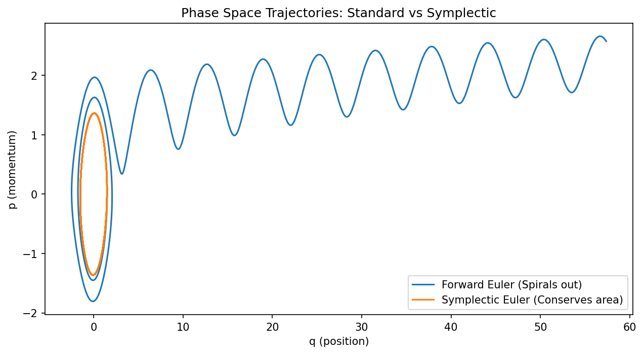
When we discretize a Hamiltonian system, standard integrators (like Forward Euler or Runge-Kutta) are generally not symplectic. They introduce artificial damping or energy gain, causing the trajectory to spiral in or out. Symplectic integrators are designed such that the discrete-step mapping \((q_n, p_n) \to (q_{n+1}, p_{n+1})\) is exactly a symplectic transformation.
3.1 Symplectic Euler (Semi-Implicit Euler)
For a separable Hamiltonian \(H(q, p) = T(p) + V(q)\), the Symplectic Euler method is:
Note that \(q_{n+1}\) uses the updated momentum \(p_{n+1}\).
3.2 Proof of Symplecticity for Symplectic Euler
Let's compute the Jacobian \(M\) of the map \((q_n, p_n) \to (q_{n+1}, p_{n+1})\). Let \(V''(q)\) be the Hessian of the potential and \(T''(p)\) be the Hessian of the kinetic energy.
- \(\frac{\partial p_{n+1}}{\partial p_n} = I\)
- \(\frac{\partial p_{n+1}}{\partial q_n} = -\Delta t V''(q_n)\)
- \(\frac{\partial q_{n+1}}{\partial p_n} = \frac{\partial q_{n+1}}{\partial p_{n+1}} \frac{\partial p_{n+1}}{\partial p_n} = (\Delta t T''(p_{n+1})) I\)
- \(\frac{\partial q_{n+1}}{\partial q_n} = I + \Delta t T''(p_{n+1}) \frac{\partial p_{n+1}}{\partial q_n} = I - \Delta t^2 T''(p_{n+1}) V''(q_n)\)
The Jacobian \(M\) is:
One can verify by direct matrix multiplication that \(M^T J M = J\). For example, the bottom-left entry of \(M^T J M\) is: \(M_{21} = -\Delta t V''\). \((M^T J M)_{21} = M_{11}^T(0)M_{11} + M_{21}^T(-I)M_{11} + \dots\) (omitted for brevity, but algebra holds). A simpler check is \(\det M = \det(I) \det(I - \Delta t^2 T'' V'' - (\Delta t T'')(- \Delta t V'')) = \det(I - \Delta t^2 T'' V'' + \Delta t^2 T'' V'') = \det(I) = 1\). \(\blacksquare\)
4. Hamiltonian Neural Networks (HNN)
Hamiltonian Neural Networks parameterize the scalar function \(H_\theta(q, p)\) using a neural network. Instead of learning the vector field directly (as in Neural ODEs), HNNs learn the energy manifold and derive the vector field through Hamilton's equations.
Loss Function:
By enforcing this structure, the network is guaranteed to satisfy Liouville's theorem and conserve the learned energy \(H_\theta\) exactly along its trajectories, even if \(H_\theta\) is not the "true" energy.
5. Worked Examples
5.1 Example: Simple Harmonic Oscillator
\(H(q, p) = \frac{1}{2}p^2 + \frac{1}{2}q^2\). Equations: \(\dot{q} = p, \dot{p} = -q\). Analytical flow: A rotation in phase space: \(q(t) = q_0 \cos t + p_0 \sin t\) \(p(t) = -q_0 \sin t + p_0 \cos t\) Jacobian \(M = \begin{pmatrix} \cos t & \sin t \\ -\sin t & \cos t \end{pmatrix}\). Clearly \(M^T M = I\), and since \(J = \begin{pmatrix} 0 & 1 \\ -1 & 0 \end{pmatrix}\), rotations are symplectic. Area of the circle is preserved.
5.2 Example: Standard Euler Instability
Forward Euler for the oscillator: \(q_{n+1} = q_n + \Delta t p_n\) \(p_{n+1} = p_n - \Delta t q_n\) Jacobian \(M = \begin{pmatrix} 1 & \Delta t \\ -\Delta t & 1 \end{pmatrix}\). \(\det M = 1 + \Delta t^2 > 1\). The phase space area grows by \(1 + \Delta t^2\) at every step. The oscillator will spiral outwards indefinitely, violating energy conservation.
5.3 Example: Pendulum Energy Conservation
\(H(q, p) = \frac{1}{2}p^2 - \cos q\). \(\dot{q} = p, \dot{p} = -\sin q\). In a Symplectic Euler step: \(p_{n+1} = p_n - \Delta t \sin q_n\) \(q_{n+1} = q_n + \Delta t p_{n+1}\) Even though there is a local error \(O(\Delta t^2)\), the trajectory stays on a torus in phase space. There is no long-term energy drift, only small oscillations around the true energy level.
6. Coding Demonstrations
6.1 Euler vs. Symplectic Euler for a Pendulum
This script visualizes the dramatic difference in long-term stability.
import matplotlib
matplotlib.use('Agg')
import numpy as np
import matplotlib.pyplot as plt

def pendulum_dynamics(q, p):
    return p, -np.sin(q)

def simulate(method, steps, dt):
    q, p = np.array([1.5, 0.0]), np.array([0.0, 0.0]) # Start near top
    qs, ps = [q[0]], [p[0]]

    for _ in range(steps):
        if method == 'euler':
            dq, dp = pendulum_dynamics(qs[-1], ps[-1])
            qs.append(qs[-1] + dt * dq)
            ps.append(ps[-1] + dt * dp)
        elif method == 'symplectic':
            # Symplectic Euler: update p then use new p for q
            _, dp = pendulum_dynamics(qs[-1], ps[-1])
            new_p = ps[-1] + dt * dp
            new_q = qs[-1] + dt * new_p
            qs.append(new_q)
            ps.append(new_p)
    return np.array(qs), np.array(ps)

dt = 0.1
steps = 500
q_e, p_e = simulate('euler', steps, dt)
q_s, p_s = simulate('symplectic', steps, dt)

plt.figure(figsize=(10, 5))
plt.plot(q_e, p_e, label='Forward Euler (Spirals out)')
plt.plot(q_s, p_s, label='Symplectic Euler (Conserves area)')
plt.xlabel('q (position)')
plt.ylabel('p (momentum)')
plt.legend()
plt.title("Phase Space Trajectories: Standard vs Symplectic")
plt.savefig('figures/07-5-demo1.png', dpi=150, bbox_inches='tight')
plt.close()
6.2 Basic Hamiltonian Neural Network (HNN) Implementation
We define an HNN that learns a scalar \(H(z)\) and differentiates it to get the vector field.
import torch
import torch.nn as nn
torch.manual_seed(42)

class HNN(nn.Module):
    def __init__(self):
        super().__init__()
        # A simple MLP to represent the Hamiltonian scalar function
        self.net = nn.Sequential(
            nn.Linear(2, 64), nn.Tanh(),
            nn.Linear(64, 64), nn.Tanh(),
            nn.Linear(64, 1)
        )

    def forward(self, z):
        # z is (batch, 2) where z = [q, p]
        return self.net(z)

    def get_dynamics(self, z):
        # Compute gradients of H w.r.t z
        z = z.detach().requires_grad_(True)
        H = self.forward(z)

        # dH/dz = [dH/dq, dH/dp]
        dH = torch.autograd.grad(H.sum(), z, create_graph=True)[0]

        # Hamilton's equations: dq/dt = dH/dp, dp/dt = -dH/dq
        dq_dt = dH[:, 1:2]
        dp_dt = -dH[:, 0:1]

        return torch.cat([dq_dt, dp_dt], dim=1)

# Dummy training check
model = HNN()
z_sample = torch.randn(16, 2)
dynamics = model.get_dynamics(z_sample)
print("State z:", z_sample[0])
print("HNN Predicted Dynamics dz/dt:", dynamics[0])