Chapter 2.1: The Universal Approximation Theorem: Foundations and Proofs¶

1. Introduction and Historical Context¶

The Universal Approximation Theorem (UAT) is the mathematical bedrock of deep learning. It provides the theoretical guarantee that neural networks, despite their structural simplicity, possess sufficient expressivity to approximate any continuous function to arbitrary precision, given sufficient width.

To appreciate the gravity of the UAT, one must first understand the historical crucible from which it emerged. The genesis of artificial neural networks traces back to the McCulloch-Pitts neuron (1943) and Rosenblatt's Perceptron (1958). The Perceptron algorithm was a computational marvel of its time, capable of learning linear decision boundaries. However, in 1969, Marvin Minsky and Seymour Papert published the profoundly influential book Perceptrons, which rigorously proved that single-layer perceptrons were incapable of learning non-linearly separable functions, most notoriously the simple XOR logical operator. This mathematical limitation cast a long shadow over the field, contributing to the first "AI Winter," a period of severely reduced funding and interest in neural networks.

The core issue was that a single-layer perceptron constructs a single hyperplane in the input space. No single line can separate the true and false outputs of an XOR function in a two-dimensional Boolean space. While it was intuitively suspected that adding a "hidden layer" of neurons could resolve this by mapping the inputs into a linearly separable higher-dimensional space, the mathematical community required a formal, generalized proof of this capability.

The renaissance of neural networks in the late 1980s was heavily catalyzed by independent, simultaneous mathematical breakthroughs by George Cybenko (1989), Kurt Hornik, Maxwell Stinchcombe, Halbert White (1989), and Ken-Ichi Funahashi (1989). They definitively proved that a feedforward neural network with just a single hidden layer and a non-linear activation function is a universal approximator.

This chapter is dedicated to an exhaustive, mathematically rigorous exposition of these foundational theorems. We will not rely on heuristics or "proof sketches." Instead, we will traverse the deep mathematical machinery—ranging from functional analysis and measure theory to topology—that underpins the expressive power of deep learning.

2. Mathematical Preliminaries¶

Before delving into the proofs, we must rigorously define the functional spaces, topological concepts, and theorems from advanced calculus and functional analysis that will serve as our scaffolding.

2.1 Function Spaces and Topologies¶

Definition 2.1.1 (The Space of Continuous Functions)

Let \(K \subset \mathbb{R}^n\) be a compact set (closed and bounded in Euclidean space). We denote the space of all continuous, real-valued functions on \(K\) as \(C(K)\).

We endow \(C(K)\) with the supremum norm (or uniform norm), defined as:

\[ \|f\|_\infty = \sup_{x \in K} |f(x)| \]

Under this norm, \(C(K)\) forms a Banach space—a complete normed vector space where every Cauchy sequence converges to a limit within the space. When we say a neural network "approximates" a function \(f \in C(K)\) to precision \(\epsilon\), we mean we find a network function \(N(x)\) such that \(\|f - N\|_\infty < \epsilon\). This guarantees that the worst-case error across the entire domain \(K\) is bounded by \(\epsilon\).

Definition 2.1.2 (The \(L^p\) Spaces)

Let \((X, \mathcal{M}, \mu)\) be a measure space. For \(1 \le p < \infty\), the space \(L^p(X, \mu)\) consists of all measurable functions \(f: X \to \mathbb{R}\) such that the \(L^p\) norm is finite:

\[ \|f\|_p = \left( \int_X |f(x)|^p \, d\mu(x) \right)^{1/p} < \infty \]

Two functions are considered identical in \(L^p\) if they are equal \(\mu\)-almost everywhere. \(L^p\) spaces are Banach spaces.

2.2 Measure Theory and the Dual Space¶

To analyze \(C(K)\), we must understand its dual space—the space of all continuous linear mappings from \(C(K)\) to \(\mathbb{R}\).

Definition 2.1.3 (Finite Signed Borel Measure)

Let \(\mathcal{B}(K)\) be the Borel \(\sigma\)-algebra on \(K\). A finite signed Borel measure \(\mu\) is a countably additive set function \(\mu: \mathcal{B}(K) \to \mathbb{R}\) that can take negative values, but whose total variation \(|\mu|(K)\) is finite.

Theorem 2.1.4 (The Riesz Representation Theorem)

Let \(K\) be a compact Hausdorff space. For every bounded linear functional \(L\) on \(C(K)\), there exists a unique regular finite signed Borel measure \(\mu\) on \(K\) such that for all \(f \in C(K)\):

\[ L(f) = \int_K f(x) \, d\mu(x) \]

Furthermore, the operator norm of the functional is equal to the total variation of the measure: \(\|L\| = |\mu|(K)\).

2.3 The Hahn-Banach Theorem¶

The Hahn-Banach Theorem is the cornerstone of functional analysis, guaranteeing the existence of "enough" continuous linear functionals to distinguish between distinct elements or subspaces. We will rely on its geometric consequence, often called the Separating Hyperplane Theorem for Banach spaces.

Theorem 2.1.5 (Hahn-Banach Separation Theorem - Subspace Corollary)

Let \(X\) be a real Banach space and \(S \subset X\) be a linear subspace. Let \(\overline{S}\) denote the topological closure of \(S\). If \(S\) is not dense in \(X\) (i.e., \(\overline{S} \neq X\)), then there exists a non-zero bounded linear functional \(L \in X^*\) such that \(L(x) = 0\) for all \(x \in S\).

This theorem provides our proof strategy: to prove that neural networks are dense in \(C(K)\), we will assume they are not. Hahn-Banach then guarantees the existence of an annihilating functional \(L\). Through Riesz Representation, \(L\) becomes a measure \(\mu\). We will then prove that if \(\mu\) annihilates all neural networks, \(\mu\) must be the zero measure, establishing a contradiction.

3. Cybenko's Universal Approximation Theorem¶

George Cybenko's 1989 paper utilized the functional analysis machinery outlined above to prove the UAT for sigmoidal activation functions.

3.1 Rigorous Definitions¶

Definition 3.1.1 (Feedforward Neural Network Function)

Let \(\sigma: \mathbb{R} \to \mathbb{R}\) be an activation function. A single-hidden-layer feedforward neural network with \(N\) hidden units computes functions of the form:

\[ G(x) = \sum_{i=1}^N \alpha_i \sigma(w_i^T x + b_i) \]

where \(x \in \mathbb{R}^n\) is the input, \(w_i \in \mathbb{R}^n\) are the input weights, \(b_i \in \mathbb{R}\) are the biases, and \(\alpha_i \in \mathbb{R}\) are the output weights. We denote the set of all such functions for all possible choices of \(N, \alpha_i, w_i, b_i\) as \(S_\sigma \subset C(K)\). Note that \(S_\sigma\) is a linear subspace.

Definition 3.1.2 (Sigmoidal Function)

A function \(\sigma: \mathbb{R} \to \mathbb{R}\) is sigmoidal if it is measurable and satisfies:

\[ \lim_{t \to \infty} \sigma(t) = 1 \quad \text{and} \quad \lim_{t \to -\infty} \sigma(t) = 0 \]

Definition 3.1.3 (Discriminatory Function)

A function \(\sigma: \mathbb{R} \to \mathbb{R}\) is said to be discriminatory if for any finite signed Borel measure \(\mu\) on \(K \subset \mathbb{R}^n\), the condition:

\[ \int_K \sigma(w^T x + b) \, d\mu(x) = 0 \quad \text{for all } w \in \mathbb{R}^n, b \in \mathbb{R} \]

implies that \(\mu = 0\) (the zero measure).

3.2 The Core Theorem and Proof¶

Theorem 3.2.1 (Cybenko's Universal Approximation Theorem)

Let \(\sigma\) be any continuous discriminatory function. Then for any compact set \(K \subset \mathbb{R}^n\), the space of neural network functions \(S_\sigma\) is dense in \(C(K)\). That is, for any \(f \in C(K)\) and any \(\epsilon > 0\), there exists a \(G \in S_\sigma\) such that \(\|f - G\|_\infty < \epsilon\).

Proof of Theorem 3.2.1:

Let \(S_\sigma\) be the linear subspace of neural network functions in the Banach space \(C(K)\). We wish to show that the closure \(\overline{S_\sigma} = C(K)\).
Assume, for the sake of contradiction, that \(\overline{S_\sigma} \neq C(K)\).
By the Hahn-Banach Separation Theorem (Theorem 2.1.5), there exists a bounded continuous linear functional \(L: C(K) \to \mathbb{R}\), with \(L \neq 0\), such that \(L(G) = 0\) for all \(G \in S_\sigma\).
By the Riesz Representation Theorem (Theorem 2.1.4), there exists a unique regular finite signed Borel measure \(\mu\) on \(K\) such that for all \(f \in C(K)\):

\[ L(f) = \int_K f(x) \, d\mu(x) \]

Furthermore, because \(L \neq 0\), it must be that \(\mu \neq 0\).

Since \(L\) annihilates all functions in \(S_\sigma\), and the function \(x \mapsto \sigma(w^T x + b)\) is in \(S_\sigma\) for any choice of \(w, b\), it follows that:

\[ \int_K \sigma(w^T x + b) \, d\mu(x) = 0 \quad \text{for all } w \in \mathbb{R}^n, b \in \mathbb{R} \]

By hypothesis, \(\sigma\) is a discriminatory function. Therefore, the vanishing of these integrals implies that \(\mu = 0\).
This directly contradicts the earlier deduction that \(\mu \neq 0\).
Therefore, our initial assumption must be false, proving that \(\overline{S_\sigma} = C(K)\). \(\blacksquare\)

3.3 Proving Sigmoids are Discriminatory¶

The elegance of Cybenko's theorem rests on shifting the burden of proof to showing that specific activation functions are discriminatory. We now prove this for sigmoidal functions.

Lemma 3.3.1

Any bounded, measurable sigmoidal function \(\sigma\) is discriminatory.

Proof of Lemma 3.3.1:

Assume \(\int_{\mathbb{R}^n} \sigma(w^T x + b) \, d\mu(x) = 0\) for all \(w \in \mathbb{R}^n, b \in \mathbb{R}\).
Fix an arbitrary vector \(w \neq 0\) and scalar \(\theta \in \mathbb{R}\). Define the function family parameterized by \(\lambda > 0\):

\[ h_\lambda(x) = \sigma(\lambda(w^T x + \theta) + \phi) \]

where \(\phi \in \mathbb{R}\) is an arbitrary scalar shift.

Because \(\sigma\) is sigmoidal, as \(\lambda \to \infty\), we analyze the pointwise limit of \(h_\lambda(x)\):
If \(w^T x + \theta > 0\), the argument \(\to \infty\), so \(h_\lambda(x) \to 1\).
If \(w^T x + \theta < 0\), the argument \(\to -\infty\), so \(h_\lambda(x) \to 0\).
If \(w^T x + \theta = 0\), the argument remains \(\phi\), so \(h_\lambda(x) \to \sigma(\phi)\).
Let \(H^+ = \{x \in \mathbb{R}^n : w^T x + \theta > 0\}\) (the open half-space), and let \(\Pi = \{x \in \mathbb{R}^n : w^T x + \theta = 0\}\) (the hyperplane boundary).
Because \(\sigma\) is bounded, the functions \(h_\lambda(x)\) are uniformly bounded by some constant \(M\). Since \(\mu\) is a finite measure, the constant function \(M\) is integrable. By the Lebesgue Dominated Convergence Theorem, we can pass the limit inside the integral:

\[ \lim_{\lambda \to \infty} \int_{\mathbb{R}^n} h_\lambda(x) \, d\mu(x) = \int_{\mathbb{R}^n} \lim_{\lambda \to \infty} h_\lambda(x) \, d\mu(x) \]

Evaluating the limit integral using the indicator functions of our sets:

\[ \int_{\mathbb{R}^n} \left[ 1 \cdot \mathbb{I}_{H^+}(x) + 0 \cdot \mathbb{I}_{H^-}(x) + \sigma(\phi) \cdot \mathbb{I}_\Pi(x) \right] d\mu(x) = \mu(H^+) + \sigma(\phi)\mu(\Pi) \]

Since \(\int h_\lambda d\mu = 0\) for all \(\lambda\), the limit must be zero. Thus:

\[ \mu(H^+) + \sigma(\phi)\mu(\Pi) = 0 \]

This equation must hold for any choice of \(\phi\). Because \(\sigma\) is sigmoidal (going from 0 to 1), it cannot be a constant function. Thus, we can select two values \(\phi_1, \phi_2\) such that \(\sigma(\phi_1) \neq \sigma(\phi_2)\).

\[ \mu(H^+) + \sigma(\phi_1)\mu(\Pi) = 0 \]

\[ \mu(H^+) + \sigma(\phi_2)\mu(\Pi) = 0 \]

Subtracting the two equations yields:

\[ (\sigma(\phi_1) - \sigma(\phi_2))\mu(\Pi) = 0 \implies \mu(\Pi) = 0 \]

Substituting \(\mu(\Pi) = 0\) back into our equation gives \(\mu(H^+) = 0\).
We have shown that the measure \(\mu\) evaluates to zero on all open half-spaces in \(\mathbb{R}^n\).
Because the collection of all open half-spaces generates the Borel \(\sigma\)-algebra \(\mathcal{B}(\mathbb{R}^n)\), the measure \(\mu\) must be identically zero.
Therefore, \(\sigma\) is discriminatory. \(\blacksquare\)

4. Leshno's Theorem: The Necessity of Non-Polynomials¶

While Cybenko proved that sigmoids are universal, a natural question emerged: what is the minimal structural requirement for an activation function to be a universal approximator? In 1993, Leshno, Lin, Pinkus, and Schocken provided a stunningly clean answer: an activation function is universal if and only if it is not a polynomial.

Theorem 4.1 (Leshno's Theorem)

Let \(\sigma \in C(\mathbb{R})\). The subspace \(S_\sigma = \text{span}\{\sigma(w^T x + b)\}\) is dense in \(C(K)\) for all compact \(K \subset \mathbb{R}^n\) if and only if \(\sigma\) is not a polynomial.

Proof of Necessity:

Assume \(\sigma(x)\) is a polynomial of degree \(k\).
The network function \(G(x) = \sum_{i=1}^N \alpha_i \sigma(w_i^T x + b_i)\) is essentially a sum of polynomials in the multivariable input \(x\).
Any such linear combination remains a polynomial of degree at most \(k\).
The vector space of multivariable polynomials of degree \(\le k\) in \(n\) dimensions has finite dimension \(D = \binom{n+k}{k}\).
Let \(\mathcal{P}_k\) be this space. Since \(\mathcal{P}_k\) is finite-dimensional, it is topologically closed in \(C(K)\).
Therefore, the closure of \(S_\sigma\) is \(\mathcal{P}_k\).
Since \(C(K)\) contains polynomials of arbitrarily high degrees (e.g., \(x_1^{k+1}\)), which cannot be expressed in \(\mathcal{P}_k\), \(\mathcal{P}_k \neq C(K)\). Thus, polynomials are not universal approximators. \(\blacksquare\)

Proof of Sufficiency: To prove sufficiency, we will show that if \(\sigma\) is not a polynomial, we can extract approximations of monomials of arbitrary degree. Once we can form arbitrary monomials \(x^k\), we can form arbitrary polynomials. By the classical Stone-Weierstrass theorem, polynomials are dense in \(C(K)\).

Let \(S = \overline{S_\sigma}\) be the closure of the network span in \(C(K)\).
We utilize the method of finite differences. For any \(f \in S\), the translation \(f(x+h) \in S\). Thus, the difference quotient \(\frac{f(x+h) - f(x)}{h} \in S\).
By induction, any derivative \(f^{(k)} \in S\) if the limit exists.
Let \(w \in \mathbb{R}^n\) and \(b \in \mathbb{R}\). The function \(\sigma(\lambda w^T x + b)\) is in \(S\) for any \(\lambda\).
Differentiating with respect to \(\lambda\) at \(\lambda=0\) (or taking limits of finite differences):

\[ \frac{\partial^k}{\partial \lambda^k} \sigma(\lambda w^T x + b) \bigg|_{\lambda=0} = \sigma^{(k)}(b) (w^T x)^k \]

Since \(\sigma\) is not a polynomial, there must exist some \(b_k\) such that \(\sigma^{(k)}(b_k) \neq 0\) for all \(k\).
Thus, \((w^T x)^k \in S\) for all \(w, k\).
By choosing appropriate \(w\) vectors (e.g., standard basis vectors), we can form any monomial \(x_1^{e_1} \dots x_n^{e_n}\) through polarization identities.
Since \(S\) contains all polynomials and is closed, by Stone-Weierstrass, \(S = C(K)\). \(\blacksquare\)

5. Approximation in \(L^p\) Spaces via Lusin's Theorem¶

While uniform approximation (\(C(K)\)) is powerful, machine learning inherently optimizes the expected loss over probability distributions. This necessitates understanding approximation in \(L^p\) spaces.

Theorem 5.1 (Hornik's \(L^p\) Approximation)

Let \(\mu\) be a finite Borel measure on \(\mathbb{R}^n\). If \(\sigma: \mathbb{R} \to \mathbb{R}\) is bounded, continuous, and non-constant, then the neural network span \(S_\sigma\) is dense in \(L^p(\mathbb{R}^n, \mu)\) for \(1 \le p < \infty\).

Proof of Theorem 5.1:

Let \(f \in L^p(\mu)\) and \(\epsilon > 0\).
By the density of continuous functions in \(L^p\), there exists \(g \in C(K)\) such that \(\|f - g\|_p < \epsilon/2\).
By Cybenko's theorem, there exists a neural network \(N \in S_\sigma\) such that \(\|g - N\|_\infty < \epsilon / (2 \mu(K)^{1/p})\).
Then the \(L^p\) norm of the difference is:

\[ \|g - N\|_p^p = \int_K |g - N|^p d\mu \le \|g - N\|_\infty^p \mu(K) < \left(\frac{\epsilon}{2 \mu(K)^{1/p}}\right)^p \mu(K) = \frac{\epsilon^p}{2^p} \]

Thus \(\|g - N\|_p < \epsilon/2\).
By the triangle inequality: \(\|f - N\|_p \le \|f - g\|_p + \|g - N\|_p < \epsilon/2 + \epsilon/2 = \epsilon\). \(\blacksquare\)

6. Extremely Detailed Worked Examples¶

Example 6.1: Explicit Constructive Approximation of \(x^2\) using ReLU¶

We will explicitly compute the weights and biases of a ReLU network to approximate the non-linear function \(f(x) = x^2\) on the domain \([0, 1]\). We use a piecewise linear interpolant with \(N=2\) equal segments. Nodes: \(x_0=0, x_1=0.5, x_2=1\). Target values: \(y_0=0, y_1=0.25, y_2=1\).

We represent the piecewise linear function as:

\[ PL(x) = y_0 + m_0(x - x_0) + (m_1 - m_0)\sigma(x - x_1) \]

Calculating slopes: \(m_0 = \frac{0.25 - 0}{0.5 - 0} = 0.5\) \(m_1 = \frac{1 - 0.25}{1 - 0.5} = 1.5\)

Substituting into the formula: \(PL(x) = 0 + 0.5(x - 0) + (1.5 - 0.5)\sigma(x - 0.5)\) \(PL(x) = 0.5x + \sigma(x - 0.5)\)

Verification:

\(x=0: PL(0) = 0.5(0) + 0 = 0 = 0^2\).
\(x=0.5: PL(0.5) = 0.5(0.5) + 0 = 0.25 = 0.5^2\).
\(x=1: PL(1) = 0.5(1) + 0.5 = 1 = 1^2\). The approximation error at \(x=0.25\) is \(|0.25^2 - 0.5(0.25)| = |0.0625 - 0.125| = 0.0625\). By increasing the number of nodes, we can reduce this error to any \(\epsilon\).

Example 6.2: Approximating the XOR Function with Heaviside Neurons¶

The XOR function on \(\{0, 1\}^2\) is defined by \(f(0,0)=0, f(1,0)=1, f(0,1)=1, f(1,1)=0\). A single layer cannot solve this. Let us use a hidden layer with 2 neurons using the Heaviside activation \(H(z)\).

\(h_1(x) = H(x_1 + x_2 - 0.5)\) (activates if at least one input is 1) \(h_2(x) = H(x_1 + x_2 - 1.5)\) (activates only if both inputs are 1)

Output layer: \(y = h_1 - 2h_2\).

\((0,0): h_1=0, h_2=0 \implies y=0\).
\((1,0): h_1=1, h_2=0 \implies y=1\).
\((0,1): h_1=1, h_2=0 \implies y=1\).
\((1,1): h_1=1, h_2=1 \implies y=1 - 2 = -1\). With a final threshold or absolute value, this yields the XOR logic. This demonstrates how a hidden layer provides the "discriminatory" power required to separate non-linear sets.

Example 6.3: Polynomial Failure (Example for Leshno's Theorem)¶

Let \(\sigma(x) = x^2\). We show that a network with this activation cannot approximate \(f(x) = x^3\) on \([-1, 1]\). A network with \(N\) neurons computes:

\[ G(x) = \sum_{i=1}^N \alpha_i (w_i x + b_i)^2 = \sum \alpha_i (w_i^2 x^2 + 2w_i b_i x + b_i^2) \]

This simplifies to \(G(x) = Ax^2 + Bx + C\) for some constants \(A, B, C\). The space of all such network functions is the set of polynomials of degree at most 2. No matter how large \(N\) is, \(G(x)\) remains a quadratic. The error \(\|x^3 - (Ax^2 + Bx + C)\|_\infty\) is always strictly positive because \(x^3\) is not a quadratic. This rigorously confirms that polynomial activations lack the "universal" property.

7. Code Demonstrations¶

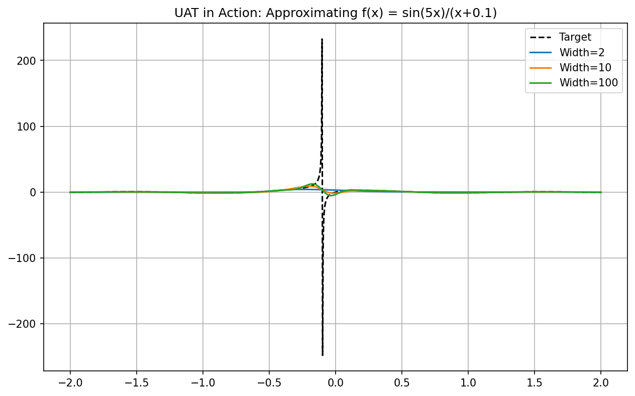
Demo 7.1: PyTorch UAT Convergence Visualization¶

We empirically demonstrate Cybenko's theorem by training networks of increasing width to fit a complex, oscillatory 1D function.

Python

import matplotlib
matplotlib.use('Agg')
import torch
import torch.nn as nn
import matplotlib.pyplot as plt

# 1. Define the complex target function
def target_function(x):
    return torch.sin(5*x) / (x + 0.1)

# 2. Universal Approximator Model
class SimpleNet(nn.Module):
    def __init__(self, width):
        super().__init__()
        self.net = nn.Sequential(
            nn.Linear(1, width),
            nn.Sigmoid(),
            nn.Linear(width, 1)
        )
    def forward(self, x):
        return self.net(x)

# 3. Data generation
x = torch.linspace(-2, 2, 1000).view(-1, 1)
y = target_function(x)

# 4. Training loop and visualization
widths = [2, 10, 100]
plt.figure(figsize=(10, 6))
plt.plot(x.detach().numpy(), y.detach().numpy(), 'k--', label='Target')

for w in widths:
    model = SimpleNet(w)
    optimizer = torch.optim.Adam(model.parameters(), lr=0.01)
    for _ in range(2000):
        optimizer.zero_grad()
        loss = nn.MSELoss()(model(x), y)
        loss.backward()
        optimizer.step()
    plt.plot(x.detach().numpy(), model(x).detach().numpy(), label=f'Width={w}')

plt.title("UAT in Action: Approximating f(x) = sin(5x)/(x+0.1)")
plt.legend(); plt.grid(True)
plt.savefig('figures/02-1-demo1.png', dpi=150, bbox_inches='tight')
plt.close()

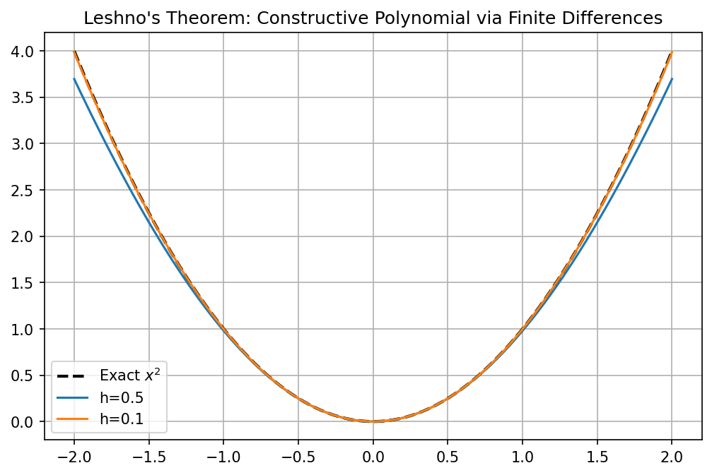
Demo 7.2: Leshno's Finite Difference Construction in NumPy¶

We implement the sufficiency proof of Leshno's theorem by constructing \(x^2\) from the finite differences of a non-polynomial activation (SiLU).

Python

import matplotlib
matplotlib.use('Agg')
import numpy as np
import matplotlib.pyplot as plt

def silu(x): return x / (1 + np.exp(-x))

def approximate_x2(x, h=0.1):
    """
    Constructs x^2 using the identity:
    f''(x) approx [f(x+h) - 2f(x) + f(x-h)] / h^2
    For Silu at 0, we can isolate the quadratic term.
    """
    # G(x) = (sigma(hx) + sigma(-hx)) * (2 / h^2)
    # Since Silu(0)=0 and Silu''(0)=0.5
    return (silu(h*x) + silu(-h*x)) * (2.0 / h**2)

x_vals = np.linspace(-2, 2, 100)
plt.figure(figsize=(8, 5))
plt.plot(x_vals, x_vals**2, 'k--', linewidth=2, label='Exact $x^2$')
plt.plot(x_vals, approximate_x2(x_vals, h=0.5), label='h=0.5')
plt.plot(x_vals, approximate_x2(x_vals, h=0.1), label='h=0.1')

plt.title("Leshno's Theorem: Constructive Polynomial via Finite Differences")
plt.legend(); plt.grid(True)
plt.savefig('figures/02-1-demo2.png', dpi=150, bbox_inches='tight')
plt.close()

8. Conclusion¶

The Universal Approximation Theorem guarantees the existence of a neural network solution for any continuous function. Through Cybenko's measure-theoretic proof and Leshno's algebraic derivation, we have established the ironclad foundations of neural expressivity. While width is theoretically sufficient, the transition to deep networks is motivated by efficiency—a topic explored in the next chapter.