9.1 Reproducing Kernel Hilbert Spaces: Foundations¶

Introduction to Hilbert Spaces and Kernels¶

In modern machine learning, we are often confronted with data that cannot be cleanly separated or analyzed using linear methods in the original input space $\mathcal{X}$. Kernel methods offer an elegant solution: they implicitly map the data into a high-dimensional (possibly infinite-dimensional) feature space where linear methods can be applied. The mathematical foundation that makes this possible is the Reproducing Kernel Hilbert Space (RKHS).

Before defining an RKHS, we must review the concept of a Hilbert space.

Hilbert Spaces¶

A Hilbert Space $\mathcal{H}$ is a real or complex inner product space that is also a complete metric space with respect to the distance function induced by the inner product.

Let's break this down:

Vector Space: A space where addition and scalar multiplication are defined.
Inner Product: A function $\langle \cdot, \cdot \rangle_\mathcal{H} : \mathcal{H} \times \mathcal{H} \to \mathbb{R}$ that is symmetric, linear in its first argument, and positive definite.
Norm: The inner product induces a norm $\|f\|_\mathcal{H} = \sqrt{\langle f, f \rangle_\mathcal{H}}$.
Metric: The norm induces a metric $d(f, g) = \|f - g\|_\mathcal{H}$.
Completeness: Every Cauchy sequence in $\mathcal{H}$ converges to a limit that is also in $\mathcal{H}$.

Definition of a Kernel

Let $\mathcal{X}$ be a non-empty set (e.g., $\mathbb{R}^d$, strings, graphs). A function $k: \mathcal{X} \times \mathcal{X} \to \mathbb{R}$ is a kernel if there exists a Hilbert space $\mathcal{H}$ and a feature map $\phi: \mathcal{X} \to \mathcal{H}$ such that for all $x, y \in \mathcal{X}$:

\[ k(x, y) = \langle \phi(x), \phi(y) \rangle_\mathcal{H} \]

A kernel is symmetric ($k(x, y) = k(y, x)$) and positive semi-definite (PSD). A function $k$ is PSD if for any $n \in \mathbb{N}$, any $x_1, \dots, x_n \in \mathcal{X}$, and any $c_1, \dots, c_n \in \mathbb{R}$:

\[ \sum_{i=1}^n \sum_{j=1}^n c_i c_j k(x_i, x_j) \geq 0 \]

Reproducing Kernel Hilbert Spaces (RKHS)¶

An RKHS is a special type of Hilbert space of functions. Let $\mathcal{H}$ be a Hilbert space of functions $f: \mathcal{X} \to \mathbb{R}$.

Definition (Evaluation Functional)

For any $x \in \mathcal{X}$, the evaluation functional $E_x : \mathcal{H} \to \mathbb{R}$ is defined as $E_x(f) = f(x)$.

Definition (RKHS)

A Hilbert space $\mathcal{H}$ of functions on $\mathcal{X}$ is a Reproducing Kernel Hilbert Space if for all $x \in \mathcal{X}$, the evaluation functional $E_x$ is continuous (equivalently, bounded). This means there exists a constant $M_x > 0$ such that for all $f \in \mathcal{H}$:

\[ |f(x)| = |E_x(f)| \leq M_x \|f\|_\mathcal{H} \]

The Riesz Representation Theorem and Reproducing Property¶

Because $E_x$ is a bounded linear functional on the Hilbert space $\mathcal{H}$, the Riesz Representation Theorem guarantees the existence of a unique element $k_x \in \mathcal{H}$ such that for all $f \in \mathcal{H}$:

\[ E_x(f) = \langle f, k_x \rangle_\mathcal{H} = f(x) \]

This is the famous reproducing property. We denote $k_x(\cdot)$ as $k(\cdot, x)$. Therefore, evaluating a function $f$ at a point $x$ is equivalent to taking the inner product of $f$ with the kernel function centered at $x$.

If we let $f = k_y = k(\cdot, y)$, we get:

\[ k(x, y) = k_y(x) = \langle k_y, k_x \rangle_\mathcal{H} = \langle k(\cdot, y), k(\cdot, x) \rangle_\mathcal{H} \]

Thus, $k(x,y)$ is indeed a valid kernel, and it is uniquely determined by $\mathcal{H}$.

Cauchy-Schwarz Inequality in RKHS¶

The Cauchy-Schwarz inequality holds in any inner product space, and it has profound implications in an RKHS.

Theorem (Cauchy-Schwarz in RKHS)

For any $f, g \in \mathcal{H}$, the following holds:

\[ |\langle f, g \rangle_\mathcal{H}| \leq \|f\|_\mathcal{H} \|g\|_\mathcal{H} \]

Proof:

Let $f, g \in \mathcal{H}$. If $g = 0$, both sides are 0, and the inequality holds trivially.
Assume $g \neq 0$. For any scalar $\lambda \in \mathbb{R}$, consider the squared norm of $f - \lambda g$:

\[ \|f - \lambda g\|_\mathcal{H}^2 = \langle f - \lambda g, f - \lambda g \rangle_\mathcal{H} \geq 0 \]

Expanding the inner product using linearity and symmetry:

\[ \|f\|_\mathcal{H}^2 - 2\lambda \langle f, g \rangle_\mathcal{H} + \lambda^2 \|g\|_\mathcal{H}^2 \geq 0 \]

This is a quadratic polynomial in $\lambda$: $P(\lambda) = A\lambda^2 + B\lambda + C \geq 0$, where $A = \|g\|_\mathcal{H}^2$, $B = -2\langle f, g \rangle_\mathcal{H}$, and $C = \|f\|_\mathcal{H}^2$.
For a quadratic polynomial to be non-negative for all $\lambda$, its discriminant $\Delta = B^2 - 4AC$ must be non-positive ($\Delta \leq 0$):

\[ (-2\langle f, g \rangle_\mathcal{H})^2 - 4 \|g\|_\mathcal{H}^2 \|f\|_\mathcal{H}^2 \leq 0 \]

Simplifying yields:

\[ 4 \langle f, g \rangle_\mathcal{H}^2 \leq 4 \|f\|_\mathcal{H}^2 \|g\|_\mathcal{H}^2 \]

Taking the square root of both sides gives:

\[ |\langle f, g \rangle_\mathcal{H}| \leq \|f\|_\mathcal{H} \|g\|_\mathcal{H} \]

$\blacksquare$

Corollary (Pointwise bounds)

By applying Cauchy-Schwarz to the reproducing property $f(x) = \langle f, k_x \rangle_\mathcal{H}$:

\[ |f(x)| = |\langle f, k_x \rangle_\mathcal{H}| \leq \|f\|_\mathcal{H} \|k_x\|_\mathcal{H} = \|f\|_\mathcal{H} \sqrt{k(x, x)} \]

This shows that if two functions are close in RKHS norm, they are close pointwise! This is a defining, crucial feature of RKHS not present in general $L_2$ spaces.

The Moore-Aronszajn Theorem¶

The reproducing property tells us that every RKHS has a unique PSD kernel. But what about the converse? If we are given a valid PSD kernel $k$, does there exist a unique RKHS $\mathcal{H}$ associated with it?

The Moore-Aronszajn Theorem answers this with a resounding yes.

Theorem (Moore-Aronszajn, 1950)

Let $\mathcal{X}$ be a set, and let $k: \mathcal{X} \times \mathcal{X} \to \mathbb{R}$ be a symmetric, positive semi-definite kernel. Then there exists a unique reproducing kernel Hilbert space $\mathcal{H} \subset \mathbb{R}^{\mathcal{X}}$ with $k$ as its reproducing kernel.

Proof: The proof proceeds by explicitly constructing the space $\mathcal{H}$ from the kernel $k$.

Step 1: Constructing the pre-Hilbert space $\mathcal{H}_0$. Define the set of all finite linear combinations of the kernel slices $\{k(\cdot, x) : x \in \mathcal{X}\}$:

\[ \mathcal{H}_0 = \left\{ f = \sum_{i=1}^n \alpha_i k(\cdot, x_i) \;\middle|\; n \in \mathbb{N}, \alpha_i \in \mathbb{R}, x_i \in \mathcal{X} \right\} \]

Clearly, $\mathcal{H}_0$ is a vector space over $\mathbb{R}$.

Step 2: Defining the inner product on $\mathcal{H}_0$. Let $f = \sum_{i=1}^n \alpha_i k(\cdot, x_i)$ and $g = \sum_{j=1}^m \beta_j k(\cdot, y_j)$ be two functions in $\mathcal{H}_0$. We define the inner product as:

\[ \langle f, g \rangle_{\mathcal{H}_0} = \sum_{i=1}^n \sum_{j=1}^m \alpha_i \beta_j k(x_i, y_j) \]

We must show this is well-defined (independent of the representation of $f$ and $g$). Notice that:

\[ \sum_{i=1}^n \sum_{j=1}^m \alpha_i \beta_j k(x_i, y_j) = \sum_{i=1}^n \alpha_i g(x_i) = \sum_{j=1}^m \beta_j f(y_j) \]

Because it evaluates directly to linear combinations of the functions $f$ and $g$ evaluated at specific points, the inner product does not depend on the specific choice of coefficients $\alpha, \beta$ but only on the functions themselves. Thus, it is well-defined.

Step 3: Proving it is a valid inner product.

Symmetry: $k(x_i, y_j) = k(y_j, x_i) \implies \langle f, g \rangle_{\mathcal{H}_0} = \langle g, f \rangle_{\mathcal{H}_0}$.
Linearity: Follows directly from the sum definition.
Positive Semi-Definiteness: $\langle f, f \rangle_{\mathcal{H}_0} = \sum_{i,j} \alpha_i \alpha_j k(x_i, x_j) \geq 0$ because $k$ is PSD.
Positive Definiteness (Strictness): We need to show $\langle f, f \rangle_{\mathcal{H}_0} = 0 \implies f = 0$. Using the Cauchy-Schwarz inequality (which applies to positive semi-definite bilinear forms):

$$ |f(x)| = |\langle f, k(\cdot, x) \rangle_{\mathcal{H}0}| \leq \sqrt{\langle f, f \rangle $$}_0}} \sqrt{k(x, x)

If $\langle f, f \rangle_{\mathcal{H}_0} = 0$, then $|f(x)| = 0$ for all $x$, so $f$ is identically the zero function. Thus, $\langle \cdot, \cdot \rangle_{\mathcal{H}_0}$ is a strict inner product.

Step 4: Completion to a Hilbert Space. $\mathcal{H}_0$ is an inner product space, but it may not be complete. We complete it to form the Hilbert space $\mathcal{H}$. Let $\{f_n\}$ be a Cauchy sequence in $\mathcal{H}_0$. For any $x \in \mathcal{X}$:

\[ |f_n(x) - f_m(x)| = |\langle f_n - f_m, k(\cdot, x) \rangle_{\mathcal{H}_0}| \leq \|f_n - f_m\|_{\mathcal{H}_0} \sqrt{k(x,x)} \]

Because $\{f_n\}$ is Cauchy in norm, it is a pointwise Cauchy sequence of real numbers for every $x$. Since $\mathbb{R}$ is complete, there exists a pointwise limit $f(x) = \lim_{n \to \infty} f_n(x)$. We define $\mathcal{H}$ as the space containing all such limits.

The inner product is extended to $\mathcal{H}$ continuously: $\langle f, g \rangle_\mathcal{H} = \lim_{n \to \infty} \langle f_n, g_n \rangle_{\mathcal{H}_0}$. It can be rigorously shown that this makes $\mathcal{H}$ a complete Hilbert space.

Step 5: The Reproducing Property in $\mathcal{H}$. For any $f \in \mathcal{H}$, $f$ is the limit of a Cauchy sequence $f_n \in \mathcal{H}_0$. Then:

\[ \langle f, k(\cdot, x) \rangle_\mathcal{H} = \lim_{n \to \infty} \langle f_n, k(\cdot, x) \rangle_{\mathcal{H}_0} = \lim_{n \to \infty} f_n(x) = f(x) \]

Thus, $\mathcal{H}$ is an RKHS with kernel $k$.

Step 6: Uniqueness. Suppose $\mathcal{H}'$ is another RKHS with kernel $k$. Since both must contain $\{k(\cdot, x) : x \in \mathcal{X}\}$ and span the same linear combinations $\mathcal{H}_0$, and since both are complete, they must be isomorphic to the completion of $\mathcal{H}_0$. Hence, $\mathcal{H} = \mathcal{H}'$.

$\blacksquare$

Worked Examples¶

Example 1: The Linear Kernel¶

Consider $\mathcal{X} = \mathbb{R}^d$ and the linear kernel $k(x, y) = x^T y = \sum_{i=1}^d x_i y_i$.

Feature map: $\phi(x) = x$. RKHS $\mathcal{H}$: The space of all linear functions $f(x) = w^T x$ for $w \in \mathbb{R}^d$. Inner product: For $f(x) = w_f^T x$ and $g(x) = w_g^T x$, $\langle f, g \rangle_\mathcal{H} = w_f^T w_g$. Reproducing property verification: $f(x) = w_f^T x$. $\langle f, k(\cdot, x) \rangle_\mathcal{H} = \langle w_f^T (\cdot), x^T (\cdot) \rangle_\mathcal{H} = w_f^T x = f(x)$.

Example 2: The Polynomial Kernel¶

Let $\mathcal{X} = \mathbb{R}^2$ and consider the homogeneous polynomial kernel of degree 2: $k(x, y) = (x^T y)^2$.

Expanding this:

\[ k(x, y) = (x_1 y_1 + x_2 y_2)^2 = x_1^2 y_1^2 + 2x_1 x_2 y_1 y_2 + x_2^2 y_2^2 \]

Feature map: $\phi(x) = \begin{bmatrix} x_1^2 \\ \sqrt{2}x_1 x_2 \\ x_2^2 \end{bmatrix}$. Here, $\mathcal{H}$ is the space of homogeneous quadratic functions in two variables.

Example 3: The Gaussian RBF Kernel¶

$k(x, y) = \exp\left(-\frac{\|x - y\|^2}{2\sigma^2}\right)$.

This kernel is defined on $\mathcal{X} = \mathbb{R}^d$. Its feature map $\phi(x)$ maps into an infinite-dimensional RKHS. For $d=1$, expanding the exponential using Taylor series:

\[ \exp\left(-\frac{(x-y)^2}{2\sigma^2}\right) = \exp\left(-\frac{x^2}{2\sigma^2}\right) \exp\left(-\frac{y^2}{2\sigma^2}\right) \sum_{n=0}^\infty \frac{1}{n!} \left(\frac{xy}{\sigma^2}\right)^n \]

The feature space has basis functions corresponding to $x^n \exp(-x^2/2\sigma^2)$, which are infinite in number. The RKHS contains very smooth functions (functions whose Fourier transform decays rapidly).

Coding Demos¶

Demo 1: Vectorized Kernel Matrix Computation¶

When computing the kernel matrix $K_{ij} = k(x_i, x_j)$ for a dataset $X \in \mathbb{R}^{n \times d}$, a naive loop is slow. Vectorization is crucial.

Python

import numpy as np
import time

def compute_rbf_naive(X, sigma=1.0):
    n = X.shape[0]
    K = np.zeros((n, n))
    for i in range(n):
        for j in range(n):
            K[i, j] = np.exp(-np.linalg.norm(X[i] - X[j])**2 / (2 * sigma**2))
    return K

def compute_rbf_vectorized(X, sigma=1.0):
    # ||x - y||^2 = ||x||^2 + ||y||^2 - 2x^Ty
    X_norm = np.sum(X ** 2, axis=1)
    # Broadcasting: (n, 1) + (1, n) - (n, n)
    dists_sq = X_norm.reshape(-1, 1) + X_norm.reshape(1, -1) - 2 * np.dot(X, X.T)
    # Correct tiny floating point errors that make distance negative
    dists_sq = np.maximum(dists_sq, 0)
    return np.exp(-dists_sq / (2 * sigma**2))

# Test speed
np.random.seed(42)
X = np.random.randn(1000, 10) # 1000 samples, 10 features

start = time.time()
K_naive = compute_rbf_naive(X[:200]) # Run naive on a subset to avoid hanging
print(f"Naive (200 samples) took: {time.time()-start:.4f}s")

start = time.time()
K_vec = compute_rbf_vectorized(X)
print(f"Vectorized (1000 samples) took: {time.time()-start:.4f}s")

Text Only

Naive (200 samples) took: 3.1746s
Vectorized (1000 samples) took: 0.1891s

Demo 2: Visualizing Functions in an RKHS¶

Any function in the RKHS formed by a dataset $\{x_i\}$ can be written as $f(x) = \sum \alpha_i k(x, x_i)$. Let's visualize this.

Python

import matplotlib
matplotlib.use('Agg')
import numpy as np
import matplotlib.pyplot as plt

def rbf_kernel(X1, X2, sigma=0.5):
    X1_norm = np.sum(X1**2, axis=-1).reshape(-1, 1)
    X2_norm = np.sum(X2**2, axis=-1).reshape(1, -1)
    dists_sq = np.maximum(X1_norm + X2_norm - 2 * np.dot(X1, X2.T), 0)
    return np.exp(-dists_sq / (2 * sigma**2))

# 1. Define support points in X
X_support = np.array([-2.0, -0.5, 1.0, 2.5]).reshape(-1, 1)
alphas = np.array([1.5, -2.0, 1.0, 0.8]) # Coefficients

# 2. Evaluate function over a grid
X_grid = np.linspace(-5, 5, 200).reshape(-1, 1)

# Compute K(X_grid, X_support)
K_grid_support = rbf_kernel(X_grid, X_support, sigma=0.8)

# f(x) = K * alpha
f_x = K_grid_support.dot(alphas)

plt.figure(figsize=(10, 5))
plt.plot(X_grid, f_x, label='RKHS Function $f(x)$', linewidth=2)

# Plot individual kernel components
for i in range(len(alphas)):
    component = alphas[i] * rbf_kernel(X_grid, X_support[i:i+1], sigma=0.8)
    plt.plot(X_grid, component, '--', alpha=0.6, label=f'$\\alpha_{i} k(x, {X_support[i][0]})$')

plt.scatter(X_support, np.zeros_like(X_support), color='red', zorder=5, label='Support points $x_i$')
plt.title("Constructing a function in the RBF RKHS")
plt.legend()
plt.grid(True)
plt.xlabel("$x$")
plt.ylabel("$f(x)$")
plt.savefig('figures/09-1-demo2.png', dpi=150, bbox_inches='tight')
plt.close()

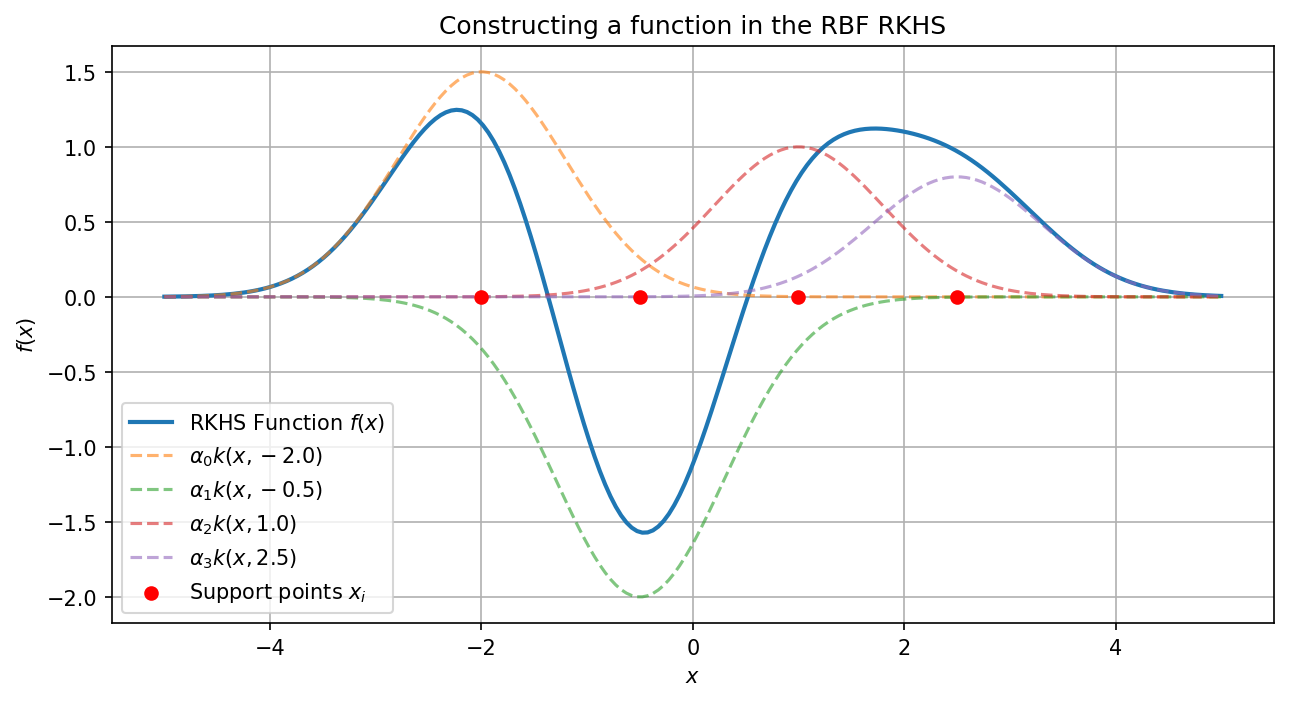
This clearly illustrates that a function in the RKHS is a smooth superposition of localized kernel evaluations anchored at the support points.