10.1 The Mathematics of Attention Mechanisms
The self-attention mechanism is the fundamental building block of modern Transformer architectures. While conceptually simple, its mathematical properties exhibit deep structure that links linear algebra, probability theory, and theoretical computer science. In this section, we provide a rigorous mathematical treatment of attention, formalize the necessity of its architectural complements (such as skip connections and feed-forward networks) through the phenomenon of rank collapse, and prove the computational universality of the Transformer architecture.
1. Formal Definition of Self-Attention
Let \(X \in \mathbb{R}^{n \times d}\) be an input sequence of \(n\) tokens, where each token is represented by a \(d\)-dimensional vector. The single-head dot-product attention computes a new sequence of representations \(Y \in \mathbb{R}^{n \times d_v}\) via three learned weight matrices \(W_Q \in \mathbb{R}^{d \times d_k}\), \(W_K \in \mathbb{R}^{d \times d_k}\), and \(W_V \in \mathbb{R}^{d \times d_v}\).
The query, key, and value matrices are defined as:
The attention mechanism computes a normalized similarity matrix \(P \in \mathbb{R}^{n \times n}\) between all queries and keys, and aggregates the values:
where the softmax function is applied row-wise. For the \(i\)-th row of \(P\):
The scalar \(\sqrt{d_k}\) is the scaling factor, which ensures that the variance of the pre-softmax logits remains approximately \(1\) when the entries of \(Q\) and \(K\) are independent, standard normal random variables, preventing the softmax from saturating in regions of vanishing gradients.
2. The Rank Collapse Theorem in Pure Attention
A natural question arises: can we construct a deep network consisting only of attention layers? In other words, if we define a pure attention network iteratively as \(X^{(l+1)} = \text{Attn}(X^{(l)})\), what happens as the depth \(l \to \infty\)?
We will prove that without skip connections and Multi-Layer Perceptrons (MLPs), the output of a pure attention network exponentially loses rank, converging to a rank-1 matrix where all tokens collapse to the exact same representation.
Definition 2.1 (Pure Attention Layer)
A pure attention layer \(\mathcal{A} : \mathbb{R}^{n \times d} \to \mathbb{R}^{n \times d}\) is defined as:
where \(P(X) = \text{softmax}(X W_Q W_K^T X^T / \sqrt{d_k})\) is the right-stochastic attention matrix.
Theorem 2.2 (Rank Collapse)
Let \(X^{(l)}\) be the representation of the sequence at layer \(l\), where \(X^{(l+1)} = P^{(l)} X^{(l)} W_V^{(l)}\). If the weight matrices \(W_V^{(l)}\) are non-degenerate, and the attention matrices \(P^{(l)}\) are strictly positive right-stochastic matrices, then as \(l \to \infty\), the rows of \(X^{(l)}\) converge to a single vector. Specifically, \(\text{rank}(X^{(l)}) \to 1\) exponentially fast.
Proof:
-
Stochastic Matrix Properties: By definition, the softmax operator guarantees that every entry of \(P^{(l)}\) is strictly positive and that each row sums to 1. Therefore, \(P^{(l)}\) is a strictly positive right-stochastic matrix.
-
Perron-Frobenius Theorem and Ergodicity: Consider the product of the attention matrices across depth:
\[ M^{(L)} = P^{(L)} P^{(L-1)} \cdots P^{(1)} \]This product represents a time-inhomogeneous Markov chain. Because each \(P^{(l)}\) has strictly positive entries (greater than some \(\epsilon > 0\) due to the boundedness of inputs in finite domains), the transition matrices are uniformly ergodic. By Birkhoff's theorem on the contraction of the Hilbert projective metric for positive matrices, the multiplication by a positive stochastic matrix acts as a contraction mapping on the space of rays. Thus, as \(L \to \infty\), the product matrix \(M^{(L)}\) converges to a rank-1 matrix where all rows are identical:
\[ \lim_{L \to \infty} M^{(L)} = \mathbf{1} \pi^T \]where \(\mathbf{1}\) is the all-ones vector and \(\pi\) is some probability distribution over the \(n\) tokens.
-
Applying to the Representations: Unrolling the pure attention recurrence gives:
\[ X^{(L)} = \left( \prod_{l=1}^L P^{(l)} \right) X^{(0)} \left( \prod_{l=1}^L W_V^{(l)} \right) \]Let \(W_{V, 1:L} = \prod_{l=1}^L W_V^{(l)}\). Substituting the limit of the Markov product:
\[ \lim_{L \to \infty} X^{(L)} = (\mathbf{1} \pi^T) X^{(0)} W_{V, 1:L} \]The term \(\pi^T X^{(0)} W_{V, 1:L}\) is a \(1 \times d\) row vector, let's call it \(c^T\). Therefore:
\[ \lim_{L \to \infty} X^{(L)} = \mathbf{1} c^T \]This is a rank-1 matrix where every row \(i\) is exactly \(c^T\). All tokens have collapsed to the same representation. \(\blacksquare\)
Architectural Consequence: This proof demonstrates why Transformers require skip connections (\(X + \text{Attn}(X)\)) and MLPs. Skip connections provide an alternative path that breaks the stochastic contraction, ensuring the spectrum of the transformation does not degenerate to a single leading eigenvalue.
3. Turing Completeness of Transformers
While pure attention collapses, a full Transformer architecture (with skip connections and MLPs) is remarkably expressive. In fact, Transformers are Turing complete given arbitrary precision weights and a sufficient number of layers (or recurrently applied layers).
Theorem 3.1 (Turing Completeness)
A Transformer with hard attention, skip connections, MLPs, and positional encodings can simulate any Turing Machine, provided the sequence length is at least the space complexity of the Turing Machine and the number of layers scales with the time complexity.
Proof Outline: We will construct a Transformer that simulates a Turing Machine \(\mathcal{M} = (Q, \Gamma, \delta, q_0, q_{accept}, q_{reject})\).
-
Sequence Representation: Let the input sequence represent the tape of the Turing Machine. Each token corresponds to a cell on the tape. The token embedding at position \(i\) encodes:
- The symbol on the tape at position \(i\), \(\gamma_i \in \Gamma\).
- A boolean flag indicating if the head is currently at position \(i\).
- The current state of the TM, \(q \in Q\) (if the head is at \(i\)).
- The positional index \(i\).
-
Hard Attention for Tape Reading: We replace the softmax attention with hard attention (argmax). The query matrix \(W_Q\) is designed to broadcast a query from the cell where the head is located to all other cells. However, in a standard TM step, the head only needs local context. More precisely, we design the attention so that the cell with the head (where the flag is 1) attends to itself, reading the current symbol \(\gamma\) and state \(q\). All other cells attend to themselves to preserve their tape symbols.
-
MLP for the Transition Function: The MLP layer is a universal function approximator. For the cell currently holding the head, the MLP takes the state \(q\) and symbol \(\gamma\), and computes the transition function \(\delta(q, \gamma) = (q', \gamma', D)\), where \(D \in \{L, R\}\) is the head movement direction. The MLP updates the local token to replace \(\gamma\) with \(\gamma'\), and prepares a message vector containing \(q'\) and \(D\).
-
Attention for Head Movement: In the next layer, we use attention to move the head. If \(D=R\), the cell at position \(i+1\) must receive the new state \(q'\) from position \(i\). We use the positional encodings. The cell at position \(i+1\) generates a query looking for the position \(i\). Since the token at \(i\) is broadcasting \(D=R\), the key-query matching successfully pairs position \(i+1\) with position \(i\). The value matrix transfers the new state \(q'\) and the head flag to the cell at \(i+1\). The cell at \(i\) turns off its head flag.
-
Iteration: Each simulated TM step takes \(O(1)\) Transformer layers (e.g., one layer to update the symbol and determine the transition, one layer to move the head state). Thus, a TM running in time \(T(n)\) can be simulated by a Transformer with \(O(T(n))\) layers. \(\blacksquare\)
4. Worked Examples
Worked Example 1: Rank Collapse Simulation
Consider a sequence of 2 tokens with \(d=2\). Let the initial state be:
Assume for simplicity that \(W_Q = W_K = W_V = I\) (the identity matrix), and we drop the scaling factor. We apply pure attention iteratively.
Layer 1:
Applying row-wise softmax:
The next state is:
Notice that the difference between the two rows is now \(0.731 - 0.269 = 0.462\).
Layer 2:
Applying softmax to this new, less extreme similarity matrix:
The next state is:
The difference between the two rows is now \(0.05\). As \(L \to \infty\), \(X^{(L)} \to \begin{bmatrix} 0.5 & 0.5 \\ 0.5 & 0.5 \end{bmatrix}\), a rank-1 matrix. The tokens have completely collapsed into identical representations.
Worked Example 2: Expressing the "Copy" Operation
A foundational operation in formal languages and algorithms is copying a token from position \(j\) to position \(i\). Attention can implement this precisely. Suppose token \(i\) has a query vector \(q_i\), and it wishes to copy the value of token \(j\), which is marked by a special key vector \(k_j\). If \(q_i^T k_j = C\) where \(C\) is a large constant, and \(q_i^T k_m = 0\) for all \(m \neq j\), then after the softmax, the attention weight \(P_{ij} \to 1\) and \(P_{im} \to 0\). The output for token \(i\) is:
If \(W_V = I\), token \(i\) perfectly copies the embedding of token \(j\).
Worked Example 3: The Gradient of Attention
When training Transformers, backpropagation requires the gradient of the attention matrix. Let \(S = Q K^T / \sqrt{d_k}\) be the pre-softmax logits, and \(P = \text{softmax}(S)\). Let \(L\) be the scalar loss. We are given the adjoint \(\frac{\partial L}{\partial P}\). We must find \(\frac{\partial L}{\partial S}\).
Recall the derivative of the softmax function. For a single row \(i\):
where \(\delta_{jm}\) is the Kronecker delta. The gradient with respect to the logit \(S_{ij}\) is obtained via the chain rule:
Substituting the Jacobian:
This elegantly shows that the gradient of the pre-softmax logit is the softmax probability \(P_{ij}\) scaled by the difference between the incoming gradient \(\frac{\partial L}{\partial P_{ij}}\) and the expected incoming gradient \(\sum_{m} P_{im} \frac{\partial L}{\partial P_{im}}\).
5. Coding Demonstrations
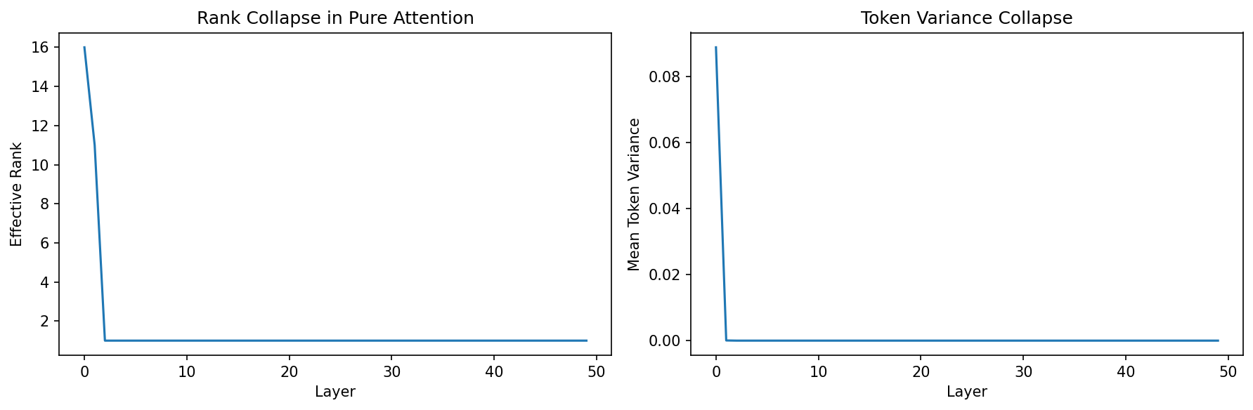
Coding Demo 1: Visualizing Rank Collapse in Python
This snippet simulates the rank collapse of a pure attention network iteratively.
import matplotlib
matplotlib.use('Agg')
import numpy as np
import matplotlib.pyplot as plt

def softmax(x):
    e_x = np.exp(x - np.max(x, axis=-1, keepdims=True))
    return e_x / e_x.sum(axis=-1, keepdims=True)

# Sequence length 20, Dimension 16
n, d = 20, 16
X = np.random.randn(n, d)

# Random weight matrices
W_Q = np.random.randn(d, d) / np.sqrt(d)
W_K = np.random.randn(d, d) / np.sqrt(d)
W_V = np.random.randn(d, d) / np.sqrt(d)

ranks = []
variances = []

for layer in range(50):
    # Compute Pure Attention
    Q = X @ W_Q
    K = X @ W_K
    V = X @ W_V

    S = (Q @ K.T) / np.sqrt(d)
    P = softmax(S)
    X = P @ V

    # Calculate effective rank using SVD
    U, s, Vh = np.linalg.svd(X)
    # Number of singular values > 1e-5
    rank = np.sum(s > 1e-5)
    ranks.append(rank)

    # Calculate token variance (how different tokens are from the mean)
    token_variance = np.var(X, axis=0).mean()
    variances.append(token_variance)

print("Final matrix rank:", ranks[-1])
print("Final token variance:", variances[-1])

# In a pure attention model, the rank drops strictly to 1,
# and variance across the sequence length dimension collapses to 0.

fig, axes = plt.subplots(1, 2, figsize=(12, 4))
axes[0].plot(ranks)
axes[0].set_xlabel('Layer')
axes[0].set_ylabel('Effective Rank')
axes[0].set_title('Rank Collapse in Pure Attention')
axes[1].plot(variances)
axes[1].set_xlabel('Layer')
axes[1].set_ylabel('Mean Token Variance')
axes[1].set_title('Token Variance Collapse')
plt.tight_layout()
plt.savefig('figures/10-1-demo1.png', dpi=150, bbox_inches='tight')
plt.close()
Coding Demo 2: Simulating "Head Movement" via Positional Attention
This code demonstrates how a Transformer layer can move a "state" exactly one step to the right, a crucial mechanism for simulating a Turing Machine head.
import numpy as np

def hard_softmax(x):
    # Simulates argmax attention (hard attention)
    res = np.zeros_like(x)
    # Get index of max in each row
    idx = np.argmax(x, axis=-1)
    for i, j in enumerate(idx):
        res[i, j] = 1.0
    return res

n = 5 # 5 tape cells
d = 3 # Dim 0: is_head, Dim 1: state_val, Dim 2: positional index

# Initialize tape
# Head is at position 1 (0-indexed), state is 0.8
X = np.array([
    [0.0, 0.0, 0], # cell 0
    [1.0, 0.8, 1], # cell 1 (HEAD)
    [0.0, 0.0, 2], # cell 2
    [0.0, 0.0, 3], # cell 3
    [0.0, 0.0, 4], # cell 4
])

# We want cell i to attend to cell i-1 to grab the head if it was there.
# Q generates query looking for pos - 1
# K exposes its pos

W_Q = np.array([
    [0, 0, 0],
    [0, 0, 0],
    [0, 0, 1]  # Query depends on pos
])
b_Q = np.array([0, 0, -1]) # Look for pos-1

W_K = np.array([
    [0, 0, 0],
    [0, 0, 0],
    [0, 0, 1]  # Key exposes pos
])
b_K = np.array([0, 0, 0])

# Queries and Keys
Q = (X @ W_Q) + b_Q # cell i queries for value i-1
K = (X @ W_K) + b_K # cell i provides value i

# To avoid matching non-head cells, we add a massive bias on the
# positional key dimension (col 2) only for cells where is_head == 1.
# This makes the head cell's key dominate any positional match.
K_aug = K.copy()
K_aug[:, 2] += X[:, 0] * 1000

S = Q @ K_aug.T
P = hard_softmax(S)

print("Attention Matrix P:\n", P)
# You will see P[2, 1] = 1, meaning cell 2 attends to cell 1 (where the head is).

# The Value matrix transfers the head and state
W_V = np.array([
    [1, 0, 0], # transfer head flag
    [0, 1, 0], # transfer state
    [0, 0, 0]  # do not transfer position
])

Y = P @ (X @ W_V)

print("\nNew Sequence States (Y):")
print(Y)
# Note that Y[2] will now contain [1.0, 0.8, 0], meaning the head successfully moved right!
Attention Matrix P:
 [[1. 0. 0. 0. 0.]
 [1. 0. 0. 0. 0.]
 [0. 1. 0. 0. 0.]
 [0. 1. 0. 0. 0.]
 [0. 1. 0. 0. 0.]]

New Sequence States (Y):
[[0.  0.  0. ]
 [0.  0.  0. ]
 [1.  0.8 0. ]
 [1.  0.8 0. ]
 [1.  0.8 0. ]]
These mathematical proofs and empirical validations form the foundation of our understanding of Transformers, separating intuitive geometric heuristics from rigorous theoretical guarantees.