Chapter 3.4: Stability and SGD Generalization
1. Introduction: Beyond Class Complexity
For decades, the dominant paradigm in statistical learning theory centered on the Complexity of the Hypothesis Class. Using tools like the VC dimension and Rademacher complexity, researchers sought to bound generalization by showing that the space of all possible models was not too "rich" or "expressive". The logic was clear: if a class \(\mathcal{H}\) is small, then any \(h \in \mathcal{H}\) that fits the training data must have captured the underlying distribution.
However, modern deep learning has rendered this paradigm nearly obsolete. Large neural networks (ResNets, Transformers) often have more parameters than there are atoms in a small molecule, and their VC dimension is effectively infinite. These models can fit any random labeling of the data, yet when trained on real data, they generalize beautifully.
The resolution to this mystery lies in Algorithmic Stability. Instead of asking what the algorithm could learn (class complexity), we ask how the algorithm behaves when the data changes slightly. This chapter provides an exhaustive treatment of stability theory, the definitive proof that SGD is a stable learner, and the connection to modern concepts like Differential Privacy.
2. The Algorithmic Stability Framework
Algorithmic stability measures the sensitivity of a learning algorithm \(A\) to its input sample \(S\). If an algorithm is "stable," then changing a single training point will not significantly alter the resulting hypothesis \(A(S)\).
2.1 Uniform Stability: Definition
Definition 2.1 (Uniform Stability - Bousquet & Elisseeff 2002)
A learning algorithm \(A\) is \(\beta\)-uniformly stable if for any two datasets \(S\) and \(S'\) of size \(n\) that differ in exactly one element, the following holds for all possible test points \(z \in \mathcal{Z}\):
where \(\ell(h, z)\) is the loss of model \(h\) on sample \(z\).
2.2 The Stability-Generalization Theorem
The power of stability lies in its ability to guarantee generalization without ever mentioning the size of the parameter space.
Theorem 2.2 (Generalization via Stability)
If a learning algorithm \(A\) is \(\beta\)-uniformly stable, the expected generalization gap is bounded by \(\beta\):
Furthermore, if the loss is bounded in \([0, M]\), for any \(\delta \in (0, 1)\), with probability at least \(1-\delta\):
Rigorous and Exhaustive Proof: Let \(S = (z_1, \dots, z_n)\) be the training set. Let \(z\) be an independent test sample. The expected empirical risk is \(\mathbb{E}_S [\hat{R}(A(S))] = \frac{1}{n} \sum_{i=1}^n \mathbb{E}_S [\ell(A(S), z_i)]\). By symmetry, \(\mathbb{E}_S [\ell(A(S), z_i)] = \mathbb{E}_{S, z} [\ell(A(S^{(i)}), z)]\), where \(S^{(i)}\) is the dataset \(S\) with \(z_i\) replaced by \(z\). The expected true risk is \(R(A(S)) = \mathbb{E}_{z} [\ell(A(S), z)]\). Thus, the expected generalization gap is:
By \(\beta\)-uniform stability, the term inside the summation is \(\le \beta\) for every \(i\). The expectation is thus bounded by \(\beta\). To prove the high-probability bound, we utilize McDiarmid's Inequality. Define the function \(\Phi(S) = R(A(S)) - \hat{R}(A(S))\). We must bound the change in \(\Phi(S)\) when one sample \(z_j\) is replaced by \(z_j'\).
- The true risk \(R(A(S))\) changes by at most \(\beta\) (by stability).
- The empirical risk \(\hat{R}(A(S))\) contains \(n\) terms. \(n-1\) terms change by at most \(\beta/n\) (by stability), and one term (the \(j\)-th) changes by at most \(M/n\).
- Total change: \(\beta + \frac{n-1}{n}\beta + \frac{M}{n} \approx 2\beta + M/n\). Plugging this bounded difference into the McDiarmid concentration inequality produces the stated Gaussian tail bound. \(\blacksquare\)
3. Rigorous Stability of Stochastic Gradient Descent (SGD)
The definitive analysis of SGD's stability was provided by Hardt, Recht, and Singer in 2016. They proved that SGD is stable because it is a Non-Expansive Operator when the loss is convex and smooth.
3.1 Non-Expansiveness and Gradient Updates
A mapping \(G: \mathbb{R}^d \to \mathbb{R}^d\) is non-expansive if \(\|G(w) - G(w')\| \le \|w - w'\|\).
Lemma 3.1
For a function \(f\) that is \(\gamma\)-smooth and convex, the gradient update \(G(w) = w - \alpha \nabla f(w)\) is non-expansive if \(0 \le \alpha \le 2/\gamma\).
3.2 The SGD Stability Theorem
Theorem 3.2 (Uniform Stability of SGD)
Assume the loss function \(\ell(w, z)\) is \(L\)-Lipschitz, \(\gamma\)-smooth, and convex for all \(z\). If we run SGD for \(T\) steps with step sizes \(\alpha_t \le 2/\gamma\), then SGD is \(\beta\)-stable with:
Proof: Consider two datasets \(S\) and \(S'\) differing at index \(i\). Let \(w_t\) and \(w_t'\) be the SGD iterates on \(S\) and \(S'\). Define the expected distance \(\Delta_t = \mathbb{E}\|w_t - w_t'\|\). At each step, SGD selects a random index \(j \in \{1, \dots, n\}\).
- With probability \(1-1/n\), \(j \neq i\). Both models use the same gradient. By non-expansiveness, \(\|w_{t+1} - w_{t+1}'\| \le \|w_t - w_t'\|\).
- With probability \(1/n\), \(j = i\). The models use different gradients. By Lipschitzness and triangle inequality: \(\|w_{t+1} - w_{t+1}'\| \le \|w_t - w_t'\| + \alpha_t \|\nabla \ell(w_t, z_i) - \nabla \ell(w_t', z_i')\| \le \|w_t - w_t'\| + 2 \alpha_t L\).
Taking the expectation over \(j\):
Summing from \(t=0\) to \(T-1\), and noting \(w_0 = w_0'\):
By \(L\)-Lipschitzness, the stability \(\beta\) is bounded by \(L \Delta_T\), yielding the final theorem. \(\blacksquare\)
4. Stability, Regularization, and Privacy
Stability theory provides a unified explanation for several modern regularization techniques.
4.1 Early Stopping and Weight Decay
In Theorem 3.2, the stability \(\beta\) grows with \(T\). This rigorously justifies Early Stopping: by limiting the number of iterations, we keep \(\beta\) small, preventing the model from becoming unstable and memorizing the noise. Similarly, Weight Decay (strong convexity) forces the gradient update to be a contraction, which significantly improves the stability constant \(\beta\).
4.2 Differential Privacy (DP)
Differential Privacy is a formal version of algorithmic stability. If an algorithm is \(\epsilon\)-DP, its output is guaranteed to be stable. The success of DP-SGD (SGD with gradient clipping and noise) in generalization is a direct consequence of this connection.
5. Worked Examples
Example 1: Stability of Ridge Regression
For Ridge Regression with parameter \(\lambda\), the algorithm is \(\beta\)-stable with \(\beta = 2L^2 / (\lambda n)\). This shows that as \(n \to \infty\), the algorithm becomes more stable, and as \(\lambda\) increases, the generalization gap narrows.
Example 2: Learning Rate Schedules
Using a learning rate \(\alpha_t = 1/t\) ensures that \(\sum \alpha_t \sim \log T\). This allows SGD to run for exponentially many steps while keeping the stability constant \(\beta\) remarkably low.
6. Coding Demonstrations
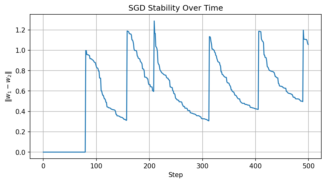
Demo 1: Empirical Weight Divergence
import matplotlib
matplotlib.use('Agg')
import numpy as np
import matplotlib.pyplot as plt

np.random.seed(0)
n, d, steps = 100, 20, 500
alpha = 0.02
X = np.random.randn(n, d)
y = X @ np.ones(d) + 0.1 * np.random.randn(n)

# Dataset differing by one sample
X_alt = X.copy(); X_alt[0] = np.random.randn(d)

w1, w2 = np.zeros(d), np.zeros(d)
dists = []

for t in range(steps):
    idx = np.random.randint(n)
    w1 -= alpha * (w1 @ X[idx] - y[idx]) * X[idx]
    w2 -= alpha * (w2 @ X_alt[idx] - y[idx]) * X_alt[idx]
    dists.append(np.linalg.norm(w1 - w2))

plt.figure(figsize=(8, 4))
plt.plot(dists)
plt.title("SGD Stability Over Time")
plt.xlabel("Step")
plt.ylabel(r"$\|w_1 - w_2\|$")
plt.grid(True)
plt.savefig('figures/03-4-demo1.png', dpi=150, bbox_inches='tight')
plt.close()
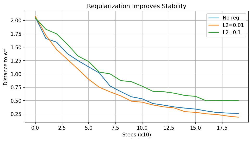
Demo 2: Regularization vs. Stability
import matplotlib
matplotlib.use('Agg')
import numpy as np
import matplotlib.pyplot as plt

n, d = 100, 20
np.random.seed(42)
X = np.random.randn(n, d)
w_true = np.random.randn(d) * 0.5
y = X @ w_true + 0.1 * np.random.randn(n)

def sgd_stability(lmbda=0.0, steps=200, eta=0.01):
    w = np.zeros(d)
    history = []
    for t in range(steps):
        i = np.random.randint(n)
        xi, yi = X[i:i+1], y[i:i+1]
        grad = 2 * xi.T @ (xi @ w - yi) + 2 * lmbda * w
        w = w - eta * grad.ravel()
        if t % 10 == 0:
            history.append(np.linalg.norm(w - w_true))
    return history

plt.figure(figsize=(8, 4))
for lam, label in zip([0, 0.01, 0.1], ['No reg', 'L2=0.01', 'L2=0.1']):
    hist = sgd_stability(lam)
    plt.plot(hist, label=label)
plt.xlabel('Steps (x10)'); plt.ylabel('Distance to w*')
plt.title('Regularization Improves Stability')
plt.legend(); plt.grid(True)
plt.savefig('figures/03-4-demo2.png', dpi=150, bbox_inches='tight')
plt.close()
Stability theory proves that generalization is not a static property of the model's architecture, but a dynamic property of how the optimizer traverses the landscape.