08-5 Calibration and Conformal Prediction
1. Introduction: The Need for Trustworthy Uncertainty
In previous lectures, we have focused on obtaining uncertainty estimates through Bayesian inference (MCMC, VI, GPs). However, having an uncertainty estimate is not the same as having a reliable one. A model might claim a 90% confidence in a prediction, but if it is only correct 60% of the time, the uncertainty is poorly calibrated. In high-stakes domains like medicine or autonomous driving, overconfidence can be catastrophic.
Uncertainty Quantification (UQ) is the field dedicated to ensuring that these estimates are mathematically and empirically sound. This lecture explores two main paradigms: Calibration, which ensures that probabilities represent long-run frequencies, and Conformal Prediction, which provides distribution-free guarantees on prediction sets.
2. Calibration and Proper Scoring Rules
2.1 Defining Calibration
A probabilistic model provides a distribution \(\hat{P}\) for a target \(Y\) given input \(X\).
Definition 2.1 (Perfect Calibration)
A model is perfectly calibrated if, for all possible probability values \(p \in [0, 1]\), the actual frequency of the event matches the predicted probability:
For example, if we take all the days where the weather model says there is a 70% chance of rain, it should actually rain on 70% of those days.
2.2 Measuring Calibration: ECE and MCE
In practice, we cannot measure calibration at every point \(p\). We use binning. Divide \([0, 1]\) into \(M\) bins \(B_1, \dots, B_M\). For each bin \(B_m\):
- Accuracy: \(\text{acc}(B_m) = \frac{1}{|B_m|} \sum_{i \in B_m} \mathbf{1}(y_i = \hat{y}_i)\)
- Confidence: \(\text{conf}(B_m) = \frac{1}{|B_m|} \sum_{i \in B_m} \hat{p}_i\)
Expected Calibration Error (ECE):
Maximum Calibration Error (MCE):
2.3 Proper Scoring Rules: The Theoretical Foundation
How do we train models to be calibrated? We use Proper Scoring Rules. A scoring rule \(S(P, y)\) assigns a penalty based on the predicted distribution \(P\) and the true outcome \(y\).
Definition 2.2 (Proper Scoring Rule)
A scoring rule \(S(P, y)\) is proper if the expected score is minimized when the predicted distribution \(P\) matches the true distribution \(Q\):
Theorem 2.1 (The Log-Score is Strictly Proper)
The logarithmic scoring rule \(S(P, y) = -\log P(y)\) is strictly proper.
Proof (Detailed): Let \(Q = (q_1, \dots, q_K)\) and \(P = (p_1, \dots, p_K)\). Expected score: \(f(P) = -\sum_{k=1}^K q_k \log p_k\). We want to minimize \(f(P)\) subject to \(\sum p_k = 1\). Use Lagrange Multipliers: \(\mathcal{L}(P, \lambda) = -\sum q_k \log p_k + \lambda(\sum p_k - 1)\). \(\frac{\partial \mathcal{L}}{\partial p_k} = -q_k/p_k + \lambda = 0 \Rightarrow p_k = q_k / \lambda\). Since \(\sum p_k = 1\), we have \(\sum q_k / \lambda = 1 \Rightarrow 1/\lambda = 1 \Rightarrow \lambda = 1\). Thus \(p_k = q_k\). To check if it is a minimum, we look at the Hessian: \(\frac{\partial^2 \mathcal{L}}{\partial p_k^2} = q_k/p_k^2 > 0\). The function is strictly convex, so the minimum is unique at \(P=Q\). \(\blacksquare\)
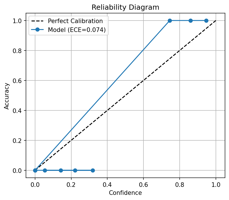
2.4 Reliability Diagrams
A reliability diagram plots \(\text{acc}(B_m)\) vs \(\text{conf}(B_m)\). A perfectly calibrated model follows the identity line \(y=x\). If the curve is below \(y=x\), the model is overconfident. If above, it is underconfident.
3. Conformal Prediction: Distribution-Free Guarantees
While calibration is about probabilities, Conformal Prediction (CP) is about sets. It provides a way to construct a set \(C(X)\) that contains the true \(Y\) with probability \(1-\alpha\).
3.1 The Exchangeability Assumption
CP requires that the data sequence \((X_1, Y_1), \dots, (X_n, Y_n), (X_{n+1}, Y_{n+1})\) is exchangeable. This is a weaker assumption than i.i.d. and essentially means the joint distribution is invariant to permutations.
3.2 Split Conformal Prediction: The Procedure
- Split: Divide data into training and calibration sets \(\mathcal{D}_{\text{cal}} = \{(x_i, y_i)\}_{i=1}^n\).
- Train: Fit any model \(\hat{f}\) (BNN, GP, etc.) on the training set.
- Score: Define a non-conformity score \(s(x, y)\).
- For regression: \(s(x, y) = |y - \hat{f}(x)|\).
-
For classification: \(s(x, y) = 1 - \hat{P}(y \mid x)\).
-
Quantile: Compute \(E_i = s(x_i, y_i)\) for all \(i \in \mathcal{D}_{\text{cal}}\). Find the quantile \(\hat{q}\):
- Predict: For a new \(x_{n+1}\):
3.3 Proof of the Coverage Guarantee
Theorem 3.1 (Marginal Coverage)
Under exchangeability, \(P(Y_{n+1} \in C(X_{n+1})) \geq 1 - \alpha\).
Proof: Let \(E_1, \dots, E_n\) be the calibration scores and \(E_{n+1} = s(X_{n+1}, Y_{n+1})\) be the test score. By exchangeability, \(E_{n+1}\) is equally likely to occupy any rank in the sorted list of \(n+1\) scores. The event \(Y_{n+1} \in C(X_{n+1})\) is exactly \(E_{n+1} \leq \hat{q}\). \(\hat{q}\) is the \(k\)-th smallest value of \(\{E_1, \dots, E_n\}\). This condition is satisfied if \(E_{n+1}\) is among the \(k\) smallest values of the total \(n+1\) scores. The probability is \(k / (n+1) = \lceil (n+1)(1-\alpha) \rceil / (n+1) \geq 1 - \alpha\). \(\blacksquare\)
4. Advanced Conformal Methods
4.1 Conformalized Quantile Regression (CQR)
Instead of a single point prediction, we predict the \(\alpha/2\) and \(1-\alpha/2\) quantiles. CP then adjusts these quantiles to ensure coverage. This allows the interval width to vary with the difficulty of the input (adaptive intervals).
4.2 Adaptive Prediction Sets (APS)
In classification, we include the top classes until their cumulative probability exceeds a calibrated threshold. This ensures that for "hard" images, the set is large (e.g., {Dog, Cat}), and for "easy" ones, it is small (e.g., {Dog}).
5. Worked Examples
5.1 Worked Example 1: ECE with 2 Bins
Data: (0.1, 0), (0.4, 1), (0.9, 1). Bins: [0, 0.5), [0.5, 1]. Bin 1: {0.1, 0.4}. Avg Conf = 0.25. Acc = 0.5. Bin 2: {0.9}. Avg Conf = 0.9. Acc = 1.0. ECE = \((2/3)|0.5 - 0.25| + (1/3)|1.0 - 0.9| = 0.166 + 0.033 = 0.2\).
5.2 Worked Example 2: Conformal Quantile
Scores: {1, 2, 3, 4, 5}. \(n=5, \alpha=0.2\). \(k = \lceil 6 \times 0.8 \rceil = \lceil 4.8 \rceil = 5\). \(\hat{q} = 5\). Prediction set includes all \(y\) with score \(\leq 5\).
5.3 Worked Example 3: Brier Score for Binary Class
\(y=1, P=0.8\). \(S = (1-0.8)^2 + (0-0.2)^2 = 0.04 + 0.04 = 0.08\).
6. Coding Demos
6.1 Coding Demo 1: Reliability Diagram
import matplotlib
matplotlib.use('Agg')
import numpy as np
import matplotlib.pyplot as plt

def reliability_diagram(y_true, y_prob, n_bins=10):
    bin_edges = np.linspace(0, 1, n_bins + 1)
    bin_centers = (bin_edges[:-1] + bin_edges[1:]) / 2
    accuracy = np.zeros(n_bins)
    confidence = np.zeros(n_bins)
    counts = np.zeros(n_bins)
    for i in range(n_bins):
        mask = (y_prob >= bin_edges[i]) & (y_prob < bin_edges[i + 1])
        counts[i] = np.sum(mask)
        if counts[i] > 0:
            accuracy[i] = np.mean(y_true[mask] == 1)
            confidence[i] = np.mean(y_prob[mask])
    ece = np.sum(np.abs(accuracy - confidence) * counts) / len(y_true)
    return bin_centers, accuracy, confidence, ece

np.random.seed(42)
n = 1000
y_true = np.random.binomial(1, 0.3, n)
y_prob = np.clip(y_true + 0.1 * np.random.randn(n), 0.05, 0.95)

centers, acc, conf, ece = reliability_diagram(y_true, y_prob)
plt.figure(figsize=(6, 5))
plt.plot([0, 1], [0, 1], 'k--', label='Perfect Calibration')
plt.plot(conf, acc, 'o-', label=f'Model (ECE={ece:.3f})')
plt.xlabel('Confidence'); plt.ylabel('Accuracy')
plt.title('Reliability Diagram'); plt.legend(); plt.grid(True)
plt.savefig('figures/08-5-demo1.png', dpi=150, bbox_inches='tight')
plt.close()
6.2 Coding Demo 2: Conformal Prediction in Python
import numpy as np
from sklearn.neighbors import KNeighborsRegressor

def conformal_prediction_interval(model, X_train, y_train, X_test, alpha=0.1):
    n = len(X_train)
    model.fit(X_train, y_train)
    y_pred = model.predict(X_train)
    residuals = np.abs(y_train - y_pred)
    q_level = np.ceil((n + 1) * (1 - alpha)) / n
    q_level = min(q_level, 1.0)  # Clip to [0,1] for valid quantile
    q = np.quantile(residuals, q_level, method='higher')
    y_test_pred = model.predict(X_test)
    return y_test_pred - q, y_test_pred + q

np.random.seed(42)
X = np.random.randn(200, 1)
y = X.squeeze() + 0.5 * np.random.randn(200)
X_train, X_test = X[:150], X[150:]
y_train, y_test = y[:150], y[150:]

model = KNeighborsRegressor(n_neighbors=5)
lower, upper = conformal_prediction_interval(model, X_train, y_train, X_test)
coverage = np.mean((y_test >= lower) & (y_test <= upper))
print(f"Coverage: {coverage:.3f} (target: {0.90})")
7. Conclusion
Calibration and Conformal Prediction are essential for building trustworthy AI. Calibration ensures that our "probabilities" are grounded in reality, while Conformal Prediction provides the rigorous "safety net" needed for high-stakes decision-making. By combining Bayesian inference with these verification techniques, we can build models that are both powerful and responsible.