4.2 Spectral Laws of Random Matrix Theory
Introduction
Random Matrix Theory (RMT) studies the properties of matrices whose entries are drawn from probability distributions. In deep learning, RMT models the Hessian of the loss landscape, the Jacobian of the network mappings, and the covariance matrices of data representations. As the dimension \(N \to \infty\), the empirical spectral distribution (ESD) of these matrices converges deterministically to specific laws.
The Stieltjes Transform
The Stieltjes transform is a powerful analytic tool for studying the spectral measure of large random matrices. For a probability measure \(\mu\) on \(\mathbb{R}\), its Stieltjes transform is defined for \(z \in \mathbb{C} \setminus \mathbb{R}\) as:
Theorem 4.2.1 (Stieltjes Inversion Formula)
The measure \(\mu\) can be recovered from \(m_\mu(z)\) by taking the limit near the real axis:
Proof: By definition, \(\text{Im} (m_\mu(x + i\epsilon)) = \int \frac{\epsilon}{(\lambda - x)^2 + \epsilon^2} d\mu(\lambda)\). This is the convolution of \(\mu\) with the Poisson kernel. As \(\epsilon \to 0\), the Poisson kernel converges weakly to the Dirac delta function \(\delta(x - \lambda)\), thus recovering the density of \(\mu\). \(\blacksquare\)
Wigner's Semicircle Law
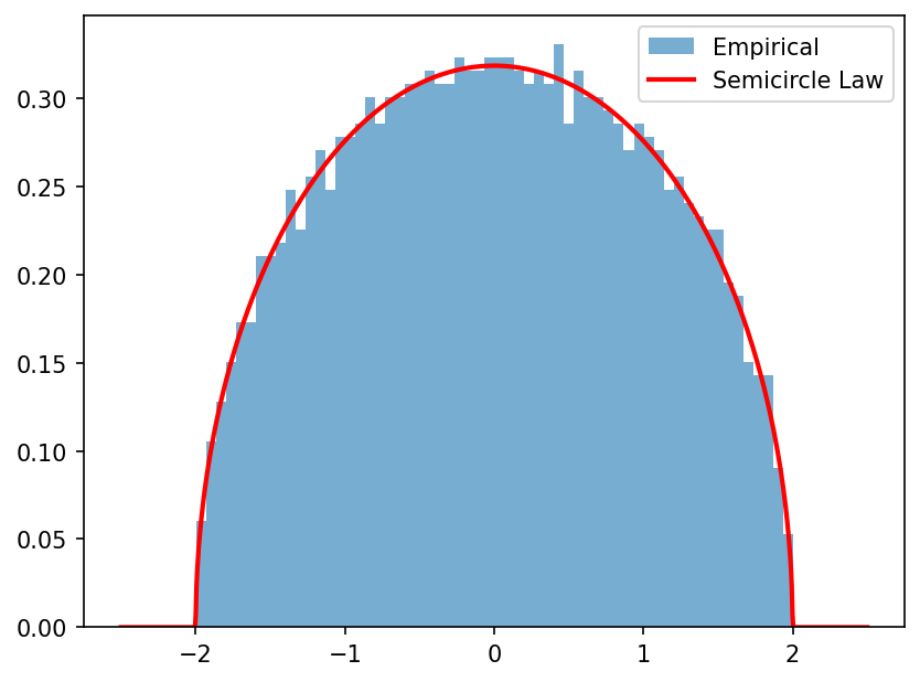
For an \(N \times N\) Wigner matrix \(W\) (symmetric, independent zero-mean entries with variance \(1/N\)), the ESD converges to the Semicircle Law.
Theorem 4.2.2 (Semicircle Law via Stieltjes Transform)
The Stieltjes transform \(m(z)\) of the semicircle distribution satisfies the quadratic equation:
Proof: Let \(G(z) = (W - zI)^{-1}\) be the resolvent. By Schur's complement formula, the diagonal entry \(G_{ii}(z)\) is given by:
where \(W^{(i)}\) is the matrix with the \(i\)-th row and column removed, and \(\alpha_i\) is the \(i\)-th column without \(W_{ii}\). As \(N \to \infty\), by the law of large numbers, the quadratic form \(\alpha_i^T (W^{(i)} - zI)^{-1} \alpha_i\) concentrates around its trace, which is \(\frac{1}{N} \text{Tr}(W^{(i)} - zI)^{-1} \approx m(z)\). Since \(W_{ii} \to 0\) in probability, we get \(m(z) = \frac{1}{-z - m(z)}\), yielding the quadratic equation \(m(z)^2 + z m(z) + 1 = 0\). Solving for \(m(z)\) and applying the inversion formula yields the density \(\rho(\lambda) = \frac{1}{2\pi} \sqrt{4 - \lambda^2}\) for \(\lambda \in [-2, 2]\). \(\blacksquare\)
The BBP Phase Transition
The Baik-Ben Arous-Péché (BBP) phase transition describes the behavior of the largest eigenvalue of a spiked covariance matrix.
Theorem 4.2.3 (BBP Phase Transition)
Let \(X \in \mathbb{R}^{N \times T}\) have i.i.d. \(\mathcal{N}(0, 1)\) entries. Consider the spiked covariance matrix \(S = \frac{1}{T} (X + \theta u v^T)(X + \theta u v^T)^T\), where \(u, v\) are unit vectors and \(\theta > 0\) is the spike strength. Let \(\gamma = N/T \le 1\). If \(\theta \le \theta_c = \gamma^{1/4}\), the largest eigenvalue \(\lambda_{\max}\) adheres to the Marchenko-Pastur edge. If \(\theta > \theta_c\), \(\lambda_{\max}\) separates from the bulk.
Proof: The matrix \(S\) is a rank-1 perturbation of a sample covariance matrix. The eigenvalues of \(S\) satisfy the secular equation \(\det(S - \lambda I) = 0\). Using the Sherman-Morrison formula on the resolvent \(G(\lambda) = (\frac{1}{T}XX^T - \lambda I)^{-1}\), the outlier eigenvalue must satisfy:
By concentration of measure, \(u^T G(\lambda) u\) converges to the Stieltjes transform of the Marchenko-Pastur law, \(m_{MP}(\lambda)\). The condition for an outlier to exist outside the support \([(1-\sqrt{\gamma})^2, (1+\sqrt{\gamma})^2]\) is that \(1/\theta^2\) must intersect the graph of \(m_{MP}(\lambda)\). The maximum value of \(m_{MP}(\lambda)\) outside the support occurs exactly at the upper edge \(\lambda_+ = (1+\sqrt{\gamma})^2\), where \(m_{MP}(\lambda_+) = 1/\sqrt{\gamma}\). Thus, for an intersection to occur, we need \(1/\theta^2 < 1/\sqrt{\gamma}\), which simplifies to \(\theta > \gamma^{1/4}\). \(\blacksquare\)
The Circular Law
For non-Hermitian random matrices \(X \in \mathbb{R}^{N \times N}\) with i.i.d. entries scaled by \(1/\sqrt{N}\), the eigenvalues converge to the uniform distribution on the unit disk in \(\mathbb{C}\).
Theorem 4.2.4 (Circular Law)
The ESD of \(X\) converges to \(\mu_c = \frac{1}{\pi} \mathbf{1}_{|z| \le 1} dx dy\).
Proof: For non-Hermitian matrices, the Stieltjes transform is insufficient because the resolvent norm diverges. Instead, we use the logarithmic potential:
The empirical logarithmic potential is \(U_N(z) = -\frac{1}{N} \log \det(X - zI)\). We write \(| \det(X - zI) | = \prod_{i=1}^N \sigma_i(X - zI)\), where \(\sigma_i\) are the singular values. The singular values of \(X - zI\) are governed by the eigenvalues of the Hermitian matrix \((X - zI)(X - zI)^*\). By computing the Stieltjes transform of this Hermitian matrix and integrating, one obtains the logarithmic potential, whose Laplacian (in the complex plane) gives the uniform density on the unit disk. \(\blacksquare\)
Worked Examples
Example 1: Computing the Resolvent For a diagonal matrix \(D = \text{diag}(d_1, \dots, d_N)\), the resolvent is \(G(z) = \text{diag}(1/(d_i-z))\). The Stieltjes transform is exactly \(m_N(z) = \frac{1}{N} \sum \frac{1}{d_i - z}\), showing its role as a generalized trace.
Example 2: Spiked Model Critical Threshold In a covariance matrix where \(N=1000, T=4000\), the aspect ratio is \(\gamma = 0.25\). The BBP critical threshold is \(\theta_c = \gamma^{1/4} = 0.707\). A signal of variance \(0.8\) will be detectable, while \(0.6\) will be hidden in the bulk noise.
Example 3: Non-Hermitian Spectrum Consider an asymmetric weight matrix \(W\) in a neural network initialized with standard normal entries variance \(1/N\). The eigenvalues will uniformly cover the complex unit disk. If the network employs a strict contraction, its Jacobian spectrum must be contained entirely within the disk to ensure stability.
Coding Demos
Demo 1: Empirical Semicircle Law
import matplotlib
matplotlib.use('Agg')
import matplotlib.pyplot as plt
import numpy as np

N = 2000
W = np.random.randn(N, N)
W = (W + W.T) / np.sqrt(2 * N) # Symmetric, variance 1/N

eigenvalues = np.linalg.eigvalsh(W)
x = np.linspace(-2.5, 2.5, 1000)
semicircle = np.where(np.abs(x) <= 2, np.sqrt(np.maximum(4 - x**2, 0)) / (2 * np.pi), 0)

plt.hist(eigenvalues, bins=60, density=True, alpha=0.6, label='Empirical')
plt.plot(x, semicircle, 'r-', lw=2, label='Semicircle Law')
plt.legend()
plt.savefig('figures/04-2-demo1.png', dpi=150, bbox_inches='tight')
plt.close()
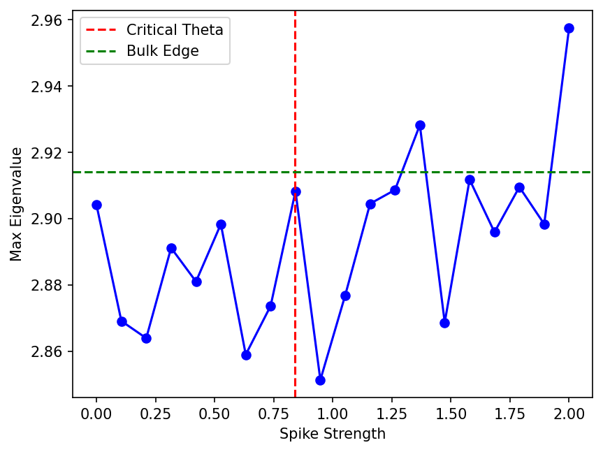
Demo 2: BBP Phase Transition Simulation
import matplotlib
matplotlib.use('Agg')
import matplotlib.pyplot as plt
import numpy as np

N, T = 500, 1000
gamma = N / T
theta_c = gamma**(0.25)
thetas = np.linspace(0, 2, 20)
max_eigs = []

for theta in thetas:
    u = np.random.randn(N, 1)
    v = np.random.randn(T, 1)
    u /= np.linalg.norm(u)
    v /= np.linalg.norm(v)

    X = np.random.randn(N, T)
    spike = theta * u @ v.T
    Y = X + spike
    S = Y @ Y.T / T
    max_eigs.append(np.linalg.eigvalsh(S).max())

edge = (1 + np.sqrt(gamma))**2
plt.plot(thetas, max_eigs, 'bo-')
plt.axvline(theta_c, color='r', linestyle='--', label='Critical Theta')
plt.axhline(edge, color='g', linestyle='--', label='Bulk Edge')
plt.xlabel('Spike Strength')
plt.ylabel('Max Eigenvalue')
plt.legend()
plt.savefig('figures/04-2-demo2.png', dpi=150, bbox_inches='tight')
plt.close()