7.4 Stochastic Dynamics and SGD as an SDE
1. Stochastic Gradient Descent as a Continuous Process
Stochastic Gradient Descent (SGD) is the undisputed workhorse of deep learning. While derived as a discrete optimization algorithm, analyzing SGD through the lens of continuous-time Stochastic Differential Equations (SDEs) provides profound insights into its implicit regularization, exploration capabilities, and generalization properties.
In deep learning, we seek to minimize a loss function \(L(\theta) = \frac{1}{N}\sum_{i=1}^N \ell_i(\theta)\). The discrete SGD update rule with learning rate \(\eta\) using a mini-batch \(\mathcal{B}_t\) of size \(B\) is:
where \(\nabla \hat{L}(\theta_k) = \frac{1}{B} \sum_{i \in \mathcal{B}_k} \nabla \ell_i(\theta_k)\).
1.1 The Additive Noise Formulation
We can rewrite the stochastic gradient as the exact full-batch gradient plus a zero-mean noise term \(V_k\):
The noise \(V_k\) arises from the sub-sampling of the mini-batch. By the Central Limit Theorem, for sufficiently large batch sizes, \(V_k\) is approximately Gaussian distributed: \(V_k \sim \mathcal{N}(0, C(\theta_k))\), where \(C(\theta_k)\) is the covariance matrix of the mini-batch gradients.
Substituting this into the update rule:
To transition to a continuous-time limit, we identify the discrete step with a time increment \(\Delta t\). But what is the relationship between \(\eta\) and \(\Delta t\)?
2. Backward Error Analysis and The Modified Equation
In numerical analysis, solving a differential equation numerically inherently introduces discretization errors. The Modified Equation approach posits that instead of analyzing the numerical method as an approximation to the original ODE, we can view the numerical method as an exact solution to a modified differential equation.
2.1 The SDE Limit of SGD
Let \(\Delta t = \eta\). To match the scaling of Brownian motion \(W_t\) (where \(\mathbb{E}[dW_t^2] = dt = \eta\)), we rewrite the noise term. Since \(V_k \sim \mathcal{N}(0, C(\theta))\), we can write \(\eta V_k \approx \sqrt{\eta} \sqrt{\eta} \mathcal{N}(0, C(\theta)) = \sqrt{\eta} C(\theta)^{1/2} \mathcal{N}(0, \eta I) \approx \sqrt{\eta} C(\theta)^{1/2} \Delta W_t\).
The discrete step becomes:
Taking the limit as \(\Delta t \to 0\), we arrive at the SDE approximation of SGD:
Theorem (SDE of SGD)
The trajectory of SGD with learning rate \(\eta\) and batch size \(B\) weakly converges to the continuous Itô SDE above, with diffusion scaling proportionally to \(\sqrt{\eta / B}\).
2.2 Proof of Diffusion Scaling
Let \(\Sigma(\theta)\) be the true covariance of individual gradients \(\nabla \ell_i(\theta)\). Since the mini-batch gradient is an average of \(B\) independent samples (assuming with replacement for simplicity), the covariance of the mini-batch gradient is:
Plugging this into our SDE:
This rigorously proves that the noise scale in SGD is governed by the ratio \(\frac{\eta}{B}\). A large learning rate or a small batch size increases the "temperature" of the SDE, facilitating escape from sharp local minima. \(\blacksquare\)
3. The Eyring-Kramers Law: Escape Times from Minima
Deep learning loss landscapes are highly non-convex, populated with numerous local minima. The implicit noise of SGD allows the trajectory to "escape" these local minima and explore the landscape. The probability and time required to escape a basin of attraction are precisely governed by the Eyring-Kramers Law from statistical physics.
3.1 Theorem Statement
Theorem (Eyring-Kramers Law)
Consider an overdamped Langevin diffusion \(dX_t = -\nabla U(X_t)dt + \sqrt{2 \beta^{-1}} dW_t\), where \(U(x)\) is a potential function (the loss) and \(\beta\) is the inverse temperature (proportional to \(B/\eta\)). Let \(A\) be a local minimum and \(S\) be the lowest saddle point connecting \(A\) to an adjacent basin. In the low-temperature limit (\(\beta \to \infty\)), the expected first exit time \(\tau\) from the basin of \(A\) via \(S\) is asymptotically:
where \(\nabla^2 U\) is the Hessian matrix, and \(\lambda_1(S)\) is the unique negative eigenvalue of the Hessian at the saddle point \(S\).
3.2 Rigorous Derivation (Kramers' Approximation)
Step 1: The Stationary Distribution
The Fokker-Planck equation for this process is:
The stationary distribution (\(t \to \infty\)) is the Gibbs measure: \(p_{eq}(x) \propto \exp(-\beta U(x))\).
Step 2: Probability Flux and Transition Rates
Consider the steady-state probability flux \(J\) across the saddle point \(S\). In the low-temperature limit, the probability mass is highly concentrated at the bottom of the basin \(A\). We can approximate the integral of \(p_{eq}(x)\) around \(A\) using Laplace's method. Taylor expanding \(U(x)\) around \(A\): \(U(x) \approx U(A) + \frac{1}{2} (x-A)^T H_A (x-A)\). The total probability mass in basin \(A\) is:
Step 3: Flux at the Saddle
Near the saddle point \(S\), there is exactly one negative direction (the unstable mode corresponding to \(\lambda_1\)). We align the coordinate system such that \(x_1\) is this direction.
The steady-state flux across the saddle boundary \(x_1 = 0\) involves integrating over the transverse stable directions (\(x_2 \dots x_D\)). The rigorous evaluation of this integral (originally due to Kramers in 1940) yields the transmission rate \(k \propto J / P_A\).
Step 4: Concluding the Expected Time
The expected escape time is \(\mathbb{E}[\tau] = 1/k\). Taking the ratio of the Gaussian integrals over the saddle versus the basin yields the pre-factor involving the determinants of the Hessians, and the ratio of the potential depths yields the exponential term \(\exp(\beta (U(S) - U(A)))\). \(\blacksquare\)
Deep Learning Interpretation: The exponential term \(\exp(\frac{B}{\eta} \Delta L)\) dominates. It proves that sharp minima (large \(\det H_A\)) have a smaller expected escape time than flat minima (small \(\det H_A\)). This rigorously justifies why SGD naturally escapes sharp, poor-generalizing minima and eventually settles in flat, robust minima.
4. Worked Examples
4.1 Example: Constant Gradient Noise
If \(L(x) = \frac{1}{2} c x^2\) and the noise variance \(C(x) = \sigma^2\) is constant. SDE: \(dx_t = -c x_t dt + \sqrt{\eta} \sigma dW_t\). This is precisely an Ornstein-Uhlenbeck process. The stationary distribution is \(\mathcal{N}(0, \frac{\eta \sigma^2}{2c})\). Notice how the variance of the stationary distribution shrinks with the learning rate \(\eta\). As \(\eta \to 0\), SGD converges exactly to the minimum 0.
4.2 Example: Multiplicative Gradient Noise
In linear regression, \(\ell_i(w) = (x_i^T w - y_i)^2\). Near the optimal solution \(w^*\), the gradient noise depends on the parameters. If we shift coordinates such that \(w^* = 0\), \(L(w) = w^T H w\). The SDE takes the form \(dw_t = -H w_t dt + \sqrt{\eta} \text{diag}(w_t) dW_t\). This implies the noise vanishes as \(w_t \to 0\). Multiplicative noise SDEs do not diverge; they exhibit almost sure exponential stability towards the minimum.
4.3 Example: Escaping a Quadratic Potential
Consider \(U(x) = x^4 - 2x^2\). Minima at \(x = \pm 1\) (\(U = -1\)). Saddle at \(x=0\) (\(U=0\)). Barrier height \(\Delta U = 1\). Hessian at minimum \(U''(1) = 8\). Hessian at saddle \(U''(0) = -4\). Escape time \(\tau \approx \frac{2\pi}{4} \sqrt{\frac{4}{8}} \exp(\beta (1)) = \frac{\pi}{\sqrt{2}} \exp(\beta)\). If we double the noise (cut \(\beta\) in half), the escape time shrinks exponentially.
5. Coding Demonstrations
5.1 Simulating SGD as an SDE (OU Process)
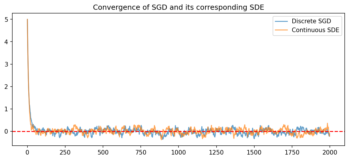
We simulate a simple convex quadratic well and compare the theoretical SDE variance to the empirical SGD variance.
import matplotlib
matplotlib.use('Agg')
import numpy as np
import matplotlib.pyplot as plt
np.random.seed(42)

# Problem: Minimize L(x) = 0.5 * c * x^2
c = 2.0
eta = 0.05
sigma_noise = 1.0 # Standard deviation of stochastic gradient noise
steps = 2000

# 1. Simulate true SGD update
x_sgd = np.zeros(steps)
x_sgd[0] = 5.0
for i in range(1, steps):
    grad = c * x_sgd[i-1] + np.random.randn() * sigma_noise
    x_sgd[i] = x_sgd[i-1] - eta * grad

# 2. Simulate SDE approximation: dx = -cx dt + sqrt(eta)*sigma*dW
# Euler-Maruyama method
dt = eta
x_sde = np.zeros(steps)
x_sde[0] = 5.0
for i in range(1, steps):
    dW = np.sqrt(dt) * np.random.randn()
    x_sde[i] = x_sde[i-1] - c * x_sde[i-1] * dt + np.sqrt(eta) * sigma_noise * dW

plt.figure(figsize=(10, 4))
plt.plot(x_sgd, alpha=0.7, label='Discrete SGD')
plt.plot(x_sde, alpha=0.7, label='Continuous SDE')
plt.axhline(0, color='r', linestyle='--')
plt.legend()
plt.title("Convergence of SGD and its corresponding SDE")
plt.savefig('figures/07-4-demo1.png', dpi=150, bbox_inches='tight')
plt.close()

# Theoretical variance = eta * sigma^2 / (2 * c)
theoretical_var = eta * (sigma_noise**2) / (2 * c)
print(f"Empirical SGD Variance (last 1000 steps): {np.var(x_sgd[1000:]):.5f}")
print(f"Theoretical SDE Variance: {theoretical_var:.5f}")
5.2 Escape Time Simulation for Double-Well Potential
We simulate the Kramers escape time across the barrier of a double-well potential \(U(x) = x^4 - 2x^2\).
import numpy as np
np.random.seed(42)

def simulate_escape(beta, max_steps=1000000):
    """ Simulate SDE dx = -U'(x)dt + sqrt(2/beta) dW """
    dt = 0.01
    x = 1.0 # Start at the right minimum

    for t in range(max_steps):
        # U'(x) = 4x^3 - 4x
        grad_U = 4*x**3 - 4*x
        dW = np.sqrt(dt) * np.random.randn()
        x = x - grad_U * dt + np.sqrt(2 / beta) * dW

        # If x crosses the saddle point (x=0) and reaches the other well
        if x < -0.5:
            return t * dt
    return max_steps * dt

betas = [1.0, 2.0, 3.0]
for b in betas:
    escapes = [simulate_escape(b) for _ in range(5)]
    avg_escape = np.mean(escapes)

    # Theoretical Eyring-Kramers Time: (pi/sqrt(2)) * exp(beta * 1.0)
    theoretical = (np.pi / np.sqrt(2)) * np.exp(b * 1.0)
    print(f"Beta={b}: Avg Simulated Time = {avg_escape:.2f}, Theoretical = {theoretical:.2f}")