The optimality of silver step sizes for gradient descent

Overview

Gradient descent can converge faster than the familiar $O(1/n)$ rate without adding momentum: a carefully arranged sequence of long and short steps achieves the silver exponent $p_{\mathrm{sil}}={\log }_2(1+\sqrt{2})\approx 1.2716$. Yuhan Ye and Kaizhao Liu prove that this exponent is optimal among predetermined nonnegative step-size schedules, up to a subpolynomial factor. They also identify the smaller optimal exponent for a single schedule that must work at every stopping horizon (Ye & Liu, 2026).

The proof constructs smooth convex functions whose gradients rotate before selected long steps. These steps pass the trajectory from one coordinate pair to the next. A recursive optimization over the selected steps reduces the lower bound to a scalar inequality containing the silver ratio. This post develops the prerequisites and the central calculations, including the correction term needed to make the recursion work and the record-time argument for the anytime result.

The primary source is Silver Rate Is (Almost) Optimal for Gradient Descent, arXiv:2609.09152v2, revised September 10, 2026. Statements and lemma numbers below refer to that version. The illustrations are original TikZ drawings; the local iterate drawing is schematic, while the gradient arc and scalar curves use the displayed formulas.

🏷️ Preliminaries: Smooth Convex Optimization

Convexity, smoothness, and the optimization model

We minimize a differentiable function $f:{\mathbb{R}}^d\to \mathbb{R}$ with at least one minimizer $x_{\ast }$. Throughout, $⟨\cdot ,\cdot ⟩$ and $\Vert \cdot \Vert$ denote the Euclidean inner product and norm.

Convexity is equivalent to the supporting-plane inequality

$$f(y)\ge f(x)+⟨\nabla f(x),y-x⟩.$$

The function is $L$-smooth if its gradient is $L$-Lipschitz:

$$\Vert \nabla f(x)-\nabla f(y)\Vert \le L\Vert x-y\Vert .$$

Integrating the gradient along the segment from $x$ to $y$ gives the corresponding upper bound

$$f(y)\le f(x)+⟨\nabla f(x),y-x⟩+\frac{L}{2}\Vert y-x{\Vert }^2.$$

These hypotheses do not require strong convexity, a unique minimizer, or a positive lower bound on curvature. The class includes objectives that are flat on entire regions. Such regions will be essential to the construction.

Given a schedule $H=(h_1,\dots ,h_n)$ with $h_t\ge 0$, gradient descent performs

$$x_t=x_{t-1}-h_t\nabla f(x_{t-1}),1\le t\le n.$$

The schedule is predetermined: it is fixed before optimization begins. It can depend on $L$ and, in the finite-horizon setting, on $n$, but it does not respond to gradients or function values observed along the trajectory. The output under study is the final iterate $x_n$.

The paper measures a schedule by its normalized worst-case error

$${\mathcal{R}}_n(H)=\underset{\begin{array}{c}d\ge 1,f\text{ convex and }L\text{-smooth}\\ x_{\ast }\in \mathrm{argmin}f,x_0\ne x_{\ast }\end{array}}{\sup }\frac{f(x_n)-f(x_{\ast })}{(L/2)\Vert x_0-x_{\ast }{\Vert }^2}.$$

The denominator is a natural scale: smoothness and $\nabla f(x_{\ast })=0$ imply

$$f(x_0)-f(x_{\ast })\le \frac{L}{2}\Vert x_0-x_{\ast }{\Vert }^2.$$

Thus ${\mathcal{R}}_n(H)$ compares error across dimensions, starting distances, and smoothness constants. A lower bound on ${\mathcal{R}}_n(H)$ says that some admissible objective and initialization make that schedule perform poorly. The hard objective may depend on the schedule and the horizon; one universal hard function is not required.

We may set $L=1$. Replacing $f$ by $f/L$ and $h_t$ by $L{h}_t$ preserves both the iterates and the normalized error. All step sizes below use this normalization; for an $L$-smooth objective, divide the dimensionless step sizes by $L$.

The classical rate and the role of long steps

For $L=1$, the constant choice $h_t=1$ gives a short proof of the familiar rate. Put $g=\nabla f(x)$ and $x^{+}=x-g$. Smoothness yields

$$f(x^{+})\le f(x)-\frac{1}{2}\Vert g{\Vert }^2.$$

Meanwhile, convexity and expansion of a squared distance give

$$\begin{array}{rl}\Vert x-x_{\ast }{\Vert }^2-\Vert x^{+}-x_{\ast }{\Vert }^2& =2⟨g,x-x_{\ast }⟩-\Vert g{\Vert }^2\\ & \ge 2(f(x)-f(x_{\ast }))-\Vert g{\Vert }^2\\ & \ge 2(f(x^{+})-f(x_{\ast })).\end{array}$$

Sum this inequality over $n$ iterations. Since function values decrease, each of the $n$ gaps on the right is at least the final gap. Consequently,

$$f(x_n)-f(x_{\ast })\le \frac{\Vert x_0-x_{\ast }{\Vert }^2}{2n},{\mathcal{R}}_n(1,\dots ,1)\le \frac{1}{n}.$$

For a general step $h$, the descent lemma instead gives

$$f(x-h\nabla f(x))\le f(x)-h\left(1-\frac{h}{2}\right)\Vert \nabla f(x){\Vert }^2.$$

When $h>2$, this inequality no longer guarantees descent. Yet occasional long steps can improve the error after a whole block of iterations. An analysis that demands progress at every individual step cannot capture this mechanism.

The silver schedule

Let

$$\rho :=1+\sqrt{2},p_{\mathrm{sil}}:={\log }_2\rho .$$

For an integer $t\ge 1$, let $v_2(t)$ be the largest integer $j\ge 0$ for which $2^j$ divides $t$. The silver schedule is

$$h_t=1+{\rho }^{v_2(t)-1}.$$

Its first seven steps are

$$\sqrt{2},2,\sqrt{2},1+\rho ,\sqrt{2},2,\sqrt{2}.$$

Write $S^{(k)}$ for its first $2^k-1$ entries. Then

$$S^{(k+1)}=(S^{(k)},1+{\rho }^{k-1},S^{(k)}),S^{(1)}=(\sqrt{2}).$$

Altschuler and Parrilo prove an $O(n^{-p_{\mathrm{sil}}})$ function-value guarantee at completed horizons $n=2^k-1$ (Altschuler & Parrilo, 2025). For any prescribed finite horizon, one can use the largest completed block that fits and append zero steps; its length is a constant fraction of the horizon, preserving the exponent. Although the silver formula defines an infinite sequence, this guarantee at completed blocks does not provide the same rate at every prefix.

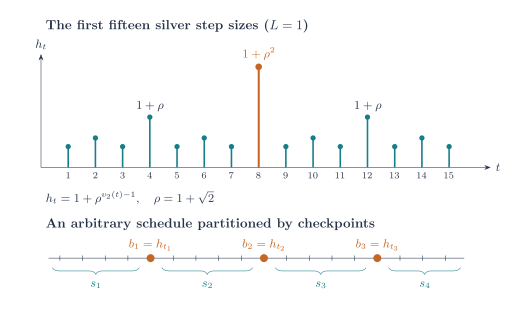
Top: the silver schedule arranges increasingly long steps at increasingly rare positions. Bottom: the lower-bound proof can select checkpoints in any schedule, with $b_i$ the selected step and $s_i$ the total of intervening steps.

Finite-horizon and anytime guarantees

In the finite-horizon, or non-anytime, problem, a different schedule may be chosen for each $n$. Its minimax error is

$$r_n^{\ast }:=\underset{H\in [0,\infty {)}^n}{\inf }{\mathcal{R}}_n(H).$$

In the anytime problem, one infinite schedule $h=(h_t{)}_{t\ge 1}$ must work for every horizon. At horizon $n$, its error is evaluated using the prefix $H_n=(h_1,\dots ,h_n)$. A guarantee must therefore survive interruption during a block, including immediately after a long step.

This distinction concerns compatibility between schedules at different horizons. The objective class and the update rule are the same in both problems.

🏷️ Main Results and Their Quantifiers

Set

$$p_{\mathrm{any}}:=\frac{2p_{\mathrm{sil}}}{1+p_{\mathrm{sil}}}\approx 1.1195,{\delta }_n:=\sqrt{\frac{\log \log n}{\log n}}.$$

Finite-horizon lower bound: Theorem 1.1

There is an absolute constant $C>0$ such that, for every sufficiently large $n$ and every predetermined nonnegative schedule $H\in [0,\infty {)}^n$,

$${\mathcal{R}}_n(H)\ge n^{-(p_{\mathrm{sil}}+C{\delta }_n)}.$$

Anytime lower bound: Theorem 1.2

There is an absolute constant $C>0$ such that every infinite predetermined nonnegative schedule has infinitely many horizons $n$ satisfying

$${\mathcal{R}}_n(H_n)\ge n^{-(p_{\mathrm{any}}+C{\delta }_n)}.$$

The first theorem holds for every schedule at each sufficiently large horizon. The second holds along infinitely many horizons for each infinite schedule; it does not assert the displayed bound at every horizon. At different horizons the supremum defining ${\mathcal{R}}_n$ may use different objectives.

The factor concealed in the changing exponent is

$$n^{-C{\delta }_n}=\exp \left(-C\sqrt{\log n\log \log n}\right).$$

It tends to zero, but more slowly than any fixed negative power of $n$. The result therefore rules out every fixed polynomial improvement over the silver exponent. It does not establish a constant-factor lower bound $\Omega (n^{-p_{\mathrm{sil}}})$, nor rule out all improvements by logarithmic factors.

Together with the silver upper bound and the anytime construction of Zhang, Lee, Du, and Chen (Zhang et al., 2025), the results determine these optimal polynomial exponents:

Method or schedule requirement	Achievable exponent	Lower-bound conclusion
Constant-step gradient descent	$1$	A baseline achievable rate
Predetermined nonnegative GD, prescribed horizon	$p_{\mathrm{sil}}\approx 1.2716$	No fixed larger exponent uniformly over objectives
One predetermined nonnegative GD schedule, all horizons	$p_{\mathrm{any}}\approx 1.1195$	No fixed larger exponent at every sufficiently large horizon
General accelerated first-order methods	$2$	A broader algorithm class, allowing auxiliary iterates

Scope of the theorem

The lower bounds concern the final iterate of ordinary GD with predetermined nonnegative step sizes on general smooth convex objectives. Adaptive schedules, negative steps, and momentum are outside this statement. The theorem also does not claim the same obstruction for restricted objective classes, such as quadratics or strongly convex functions.

🏷️ Convex-Analysis Tools for Constructing a Hard Objective

The adversary must produce a single globally defined smooth convex function whose gradients generate the desired trajectory. Drawing plausible gradient arrows is insufficient: arbitrary prescribed arrows need not be gradients of such a function. Moreau envelopes and projections supply the needed consistency.

Moreau envelopes and proximal maps

For a proper closed convex function $g:{\mathbb{R}}^d\to (-\infty ,+\infty ]$, define the following regularization. Here proper means that $g$ has at least one finite value, and closed means that its epigraph is closed.

$${\mathrm{env}}_{1}g(x)=\underset{y}{\min }\left\{g(y)+\frac{1}{2}\Vert x-y{\Vert }^2\right\},$$

and let ${\mathrm{prox}}_g(x)$ be the unique minimizing $y$. The quadratic makes the minimization strongly convex even when $g$ has corners. The envelope is differentiable, convex, and $1$-smooth, with

$$\nabla {\mathrm{env}}_{1}g(x)=x-{\mathrm{prox}}_g(x).$$

The subdifferential $\partial g(p)$ consists of vectors $v$ satisfying $g(y)\ge g(p)+⟨v,y-p⟩$ for every $y$. It replaces the gradient at a corner. For the Lipschitz property, put $p={\mathrm{prox}}_g(x)$ and $q={\mathrm{prox}}_g(y)$. Optimality gives $x-p\in \partial g(p)$ and $y-q\in \partial g(q)$. Adding the two supporting-plane inequalities gives monotonicity:

$$⟨(x-p)-(y-q),p-q⟩\ge 0.$$

If $a=(x-p)-(y-q)$, then $x-y=a+(p-q)$, so

$$\Vert a{\Vert }^2\le ⟨a,x-y⟩\le \Vert a\Vert \Vert x-y\Vert .$$

Hence the envelope’s gradient is $1$-Lipschitz. The gradient formula follows by comparing the minimizing expressions at neighboring points. These are classical properties of Moreau regularization (Moreau, 1965).

Support functions and Euclidean projection

For a nonempty compact convex set $K$, its support function is

$${\sigma }_K(z):=\underset{v\in K}{\max }⟨v,z⟩.$$

The key identity is

$$\nabla {\mathrm{env}}_1{\sigma }_K(z)={\Pi }_K(z),$$

where ${\Pi }_K$ is Euclidean projection onto $K$. Here is a direct explanation. Write $p={\Pi }_K(z)$. The projection condition is

$$⟨z-p,v-p⟩\le 0(v\in K).$$

Thus $p$ maximizes $⟨v,z-p⟩$ over $K$, giving $p\in \partial {\sigma }_K(z-p)$. This is exactly the optimality condition for $z-p$ to equal ${\mathrm{prox}}_{{\sigma }_K}(z)$. The envelope gradient is therefore $p$.

Equivalently, $z-p$ belongs to the normal cone

$$N_K(p):=\{w:⟨w,v-p⟩\le 0\text{ for every }v\in K\}.$$

This criterion will verify the gradient vectors in the construction. On a circular boundary, an outward radial vector is a normal vector.

Flat regions and the one-sided Huber function

If $g\ge 0$, its envelope has the same zero set. Indeed, $g(x)=0$ allows the candidate $y=x$ with value zero; conversely, a zero minimum forces both $g(y)=0$ and $x=y$.

This makes envelopes useful for preserving regions where a component is completely inactive. For a differentiable nonnegative function, every zero is a minimizer and has zero gradient.

The terminal component uses the one-sided Huber function

$$H_{\delta }(z)=\{\begin{array}{ll}0,& z\le 0,\\ z^2/2,& 0\le z\le \delta ,\\ \delta z-{\delta }^2/2,& z\ge \delta .\end{array}$$

Its derivative is $\min \{\delta ,\max \{z,0\}\}$, hence is $1$-Lipschitz. It is convex, $1$-smooth, flat to the left, and affine sufficiently far to the right. In the affine region, the gradient is constant, making the final loss easy to compute exactly.

🏷️ Checkpoints and the Geometric Bottleneck

Fix any schedule $h=(h_1,\dots ,h_n)$. Select indices

$$T=\{t_1<\cdots <t_k\},t_0=0,t_{k+1}=n+1,$$

and define

$$b_i=h_{t_i},s_i=\sum _{t=t_{i-1}+1}^{t_i-1}{h}_t.$$

The $b_i$ are checkpoints, typically long steps. The $s_i$ are sums of the intervening steps, not counts of iterations. In particular, $s_{k+1}$ is the sum after the final checkpoint.

Earlier constructions join one-sided Huber terms on adjacent coordinates. While a term involving $x^{(i)}-x^{(i+1)}$ is affine, its gradient is proportional to $e_i-e_{i+1}$. A GD step decreases coordinate $i$ and increases coordinate $i+1$ by equal amounts. Both changes shrink the difference keeping that term active. This double consumption of the active coordinate gap leads to a transfer ratio

$$\frac{b_i}{2(2+s_i)}$$

and, for positive step-size schedules, the checkpoint lower bound

$${\mathcal{R}}_n(h)\ge \frac{1}{4(1+s_{k+1})}\prod _{i=1}^k{\left[\frac{b_i}{2(2+s_i)}\right]}^2.$$

This is Fact 2.1 of the paper, attributed to Jung, Cho, and Yun (Jung, Cho & Yun, 2026). Its recursive analysis gives the exponent ${\log }_2(1+\sqrt{3})\approx 1.4500$. For a lower bound, a smaller exponent is stronger: $n^{-1.2716}$ is larger than $n^{-1.4500}$ at large $n$.

Ye and Liu reduce the coefficient of $s_i$ toward $1$. During much of an intervening block, the gradient points horizontally, consuming the current coordinate with little increase in the next. Near the selected step, it turns almost vertically, allowing that step to raise the next coordinate substantially.

The necessary turn must still be compatible with convexity and smoothness, and the previous component must stay inactive after the next one begins. Both requirements are built into the local objective.

🏷️ Rotating Gradients and the Two-Coordinate Construction

A circular arc in gradient space

Choose $ϵ,\gamma >0$ and set

$$c=\sqrt{1+2\gamma +{ϵ}^2},R=\sqrt{{ϵ}^2+(1+\gamma {)}^2}.$$

For $0\le q\le 1$, define

$$v(q)=(p(q),-q),p(q)=\sqrt{R^2-(q+\gamma {)}^2}.$$

These vectors run along a circle centered at $(0,\gamma )$, from

$$v(0)=(c,0)\text{to}v(1)=(ϵ,-1).$$

Let $K$ be the convex hull of this arc and the origin. The gradient of ${\mathrm{env}}_1{\sigma }_K$ is projection onto $K$, so the task becomes finding points whose projections follow the arc while respecting the GD update.

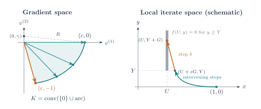
Left: an exact gradient arc with illustrative parameters $ϵ=0.22$, $\gamma =0.15$. Right: the local transfer geometry. The final gradient is proportional to $(ϵ,-1)$, so a selected step increases the second coordinate by $G$ while decreasing the first by $ϵG$. The gray ray is a certified zero set, not a claim about the full zero region.

Constructing the trajectory backward

Let ${\alpha }_1,\dots ,{\alpha }_m\ge 0$ be the local intervening steps. Fix the terminal point and gradient

$$r_m=v_m=(ϵ,-1).$$

Construct earlier points backward so that

$$r_{j-1}=r_j+{\alpha }_j{v}_{j-1},v_{j-1}={\Pi }_K(r_{j-1}).$$

The first equation is GD read backward. The second ensures that its gradient comes from one fixed smooth convex objective.

For an explicit backward step, write $r_j=(u_j,-y_j)$ and put

$${\Delta }_j=y_j+\gamma -{\alpha }_j\gamma .$$

If ${\Delta }_j\le u_j\gamma /c$, choose $v_{j-1}=(c,0)$. Otherwise, let

$$\begin{array}{rl}{D}_j& =\sqrt{u_j^2+{\Delta }_j^2},\\ v_{j-1}& =\left(\frac{R{u}_j}{D_j},\gamma -\frac{R{\Delta }_j}{D_j}\right).\end{array}$$

Here $D_j$ is only an auxiliary norm in the backward construction; the coordinate heights $D_i$ introduced later have a different role. In the curved branch, the residual is

$$r_{j-1}-v_{j-1}=\left(\frac{D_j}{R}+{\alpha }_j-1\right)(v_{j-1}-(0,\gamma )).$$

The coefficient is nonnegative, by the backward invariants $u_j\ge ϵ$ and $y_j\ge 1$ and the reverse triangle inequality. Thus this residual points along an outward normal to the circle, proving the projection condition. The horizontal branch uses the normal cone at the endpoint $(c,0)$. Appendix A.1 verifies these invariants, including $y_j/u_j\le 1/ϵ$.

Bounded displacement during the turn

Put

$$S=\sum _j{\alpha }_j,P=\sum _j{\alpha }_j{v}_{j-1}^{(1)},Q=-\sum _j{\alpha }_j{v}_{j-1}^{(2)}.$$

Lemma 3.1 establishes

$$P\le cS,0\le Q\le H(ϵ,\gamma ).$$

The first bound follows from $v^{(1)}\le c$. The second is the substantial improvement: vertical displacement is bounded independently of the total $S$. Going backward, once the gradient reaches $(c,0)$, every earlier gradient is horizontal and contributes nothing to $Q$. A short block can start partway along the arc; the same displacement bounds still hold.

To control the curved portion, define

$${\sigma }_j=\frac{y_j+\gamma }{u_j},A(\sigma )=\sigma +\sqrt{1+{\sigma }^2}.$$

In the curved branch, the recursion gives

$$\frac{u_{j-1}}{u_j}=1+\frac{R}{\gamma }\frac{{\sigma }_j-{\sigma }_{j-1}}{\sqrt{1+{\sigma }_{j-1}^2}}\le {\left[\frac{A({\sigma }_j)}{A({\sigma }_{j-1})}\right]}^{R/\gamma }.$$

The inequality follows from convexity of $A$, followed by Bernoulli’s inequality. The ratios telescope, bounding the sum of step sizes spent on the curved portion and yielding the explicit choice

$$H={\left[\frac{c(1+\gamma +R)}{ϵ(\gamma +R)}\right]}^{R/\gamma }-1.$$

This constant becomes large when the arc approaches the desired limiting geometry. Its growth will determine the subpolynomial loss in the final theorem.

A finite smooth objective with the required zero sets

The construction uses only finitely many arc vectors. Let

$$\mathcal{V}=\{0,v_0,\dots ,v_m,(c,0)\}.$$

Since $\mathrm{conv}(\mathcal{V})\subseteq K$ contains each $v_j$, a vector that is the projection of $r_j$ onto $K$ remains its projection onto this smaller set. This replaces the entire arc by a finite maximum of affine functions.

Choose

$$C_0=ϵ+\frac{1+H}{ϵ},b\ge 1+{ϵ}^{-2},A\ge C_0,$$

and put

$$\theta =\frac{1}{cS+ϵb+A},z_{\circ }=(1,0)-\theta r_0.$$

Define

$$\varphi (z)=\theta \underset{v\in \mathcal{V}}{\max }⟨v,z-z_{\circ }⟩,f={\mathrm{env}}_1\varphi .$$

Then $f$ is nonnegative, convex, and $1$-smooth, and

$$\nabla f(z_{\circ }+\theta r_j)=\theta v_j.$$

The scaling therefore preserves the prescribed GD trajectory. Writing

$$G=\theta b,U=1-\theta (P+ϵb),Y=\theta Q,$$

it gives the transfer

$$(1,0)\stackrel{{\alpha }_1,\dots ,{\alpha }_m}{\to }(U+ϵG,Y)\stackrel{b}{\to }(U,Y+G),G=\frac{b}{cS+ϵb+A}.$$

Crucially, Lemma 3.2 also guarantees

$$f(x,y)=0\text{when }x\le 0,y\ge 0,f(U,y)=0\text{when }y\ge Y.$$

For the second statement, every vector $v=(p,-q)\in \mathcal{V}$ satisfies $q\le p/ϵ$. At $(U,Y)$ its affine piece is proportional to

$$(1-b)ϵp+q\le (1-b)ϵp+\frac{p}{ϵ}\le 0.$$

Increasing $y$ only decreases that piece. Since the zero vector is also included, the maximum equals zero there, and the envelope preserves the zero set. The first zero region follows similarly from $P\le cS$, $Q\le H$, and $A\ge C_0$.

These regions make it possible to run a sequence of local components without reactivating the previous ones. Taking $ϵ=0$ prematurely would lose the horizontal motion needed for this deactivation; taking $\gamma =0$ would lose the turning mechanism.

🏷️ Joining Local Transfers into a Global Hard Function

Coordinate heights and activation levels

Return to the selected checkpoints $t_1,\dots ,t_k$. For the $i$-th component, apply the local construction with intervening steps $h_t/2$, selected step $b_i/2$, and $A=ca/2$. We choose

$$B_0=2(1+{ϵ}^{-2}),b_i\ge B_0,a\ge 2C_0/c.$$

Its transfer ratio is then

$$G_i=\frac{b_i}{c(a+s_i)+ϵb_i}.$$

The division by $2$ anticipates the factor $1/2$ in the global objective. Denote the local function and endpoint data by $f_i,U_i,Y_i$. Define recursively

$$D_1=1,{\ell }_1=0,D_{i+1}=D_i{G}_i,{\ell }_{i+1}=D_i{Y}_i.$$

Here ${\ell }_i$ is the activation level of coordinate $i$, and $D_i$ is its height above that level when component $i$ begins. The scaled component is

$${\Phi }_i(x)=D_i^2{f}_i\left(\frac{x^{(i)}-{\ell }_i}{D_i},\frac{x^{(i+1)}}{D_i}\right).$$

The factor $D_i^2$ exactly compensates for the spatial rescaling: differentiating gives a factor $D_i$, and comparing two gradients cancels that factor against the denominator $D_i$. Thus ${\Phi }_i$ remains $1$-smooth on its coordinate pair.

Set

$$F(x)=\frac{1}{2}\sum _{i=1}^k{\Phi }_i(x)+\frac{1}{2}{H}_{\delta }(x^{(k+1)}-{\ell }_{k+1}),x_0=e_1.$$

All terms are nonnegative and vanish at the origin, so $F(0)=\min F=0$. During the $i$-th block, only ${\Phi }_i$ contributes to the gradient. At its selected step, coordinate $i+1$ rises from ${\ell }_{i+1}$ to ${\ell }_{i+1}+D_{i+1}$.

The zero sets prove this sequential activation. Before a component begins, its first input is nonpositive and its second is nonnegative, so it vanishes. After component $i$ finishes, its first input remains $U_i$. The next component decreases coordinate $i+1$ but keeps it at least ${\ell }_{i+1}=D_i{Y}_i$, so the second input to $f_i$ remains at least $Y_i$. The previous component therefore stays zero.

This is a trajectory invariant, not merely a statement that components use different coordinates: neighboring components share a coordinate, and their zero sets control that interaction.

Global smoothness despite shared coordinates

A sum of $k$ arbitrary $1$-smooth functions need only be $k$-smooth. Here every coordinate appears in at most two terms. If $d=y-x$, summing the local smoothness bounds gives

$$\begin{array}{rl}F(y)& \le F(x)+⟨\nabla F(x),d⟩\\ & +\frac{1}{4}\left[\sum _{i=1}^k((d^{(i)}{)}^2+(d^{(i+1)}{)}^2)+(d^{(k+1)}{)}^2\right]\\ & \le F(x)+⟨\nabla F(x),d⟩+\frac{1}{2}\Vert d{\Vert }^2.\end{array}$$

Thus $F$ is globally $1$-smooth, independently of the number of checkpoints.

Exact final loss

At the last checkpoint, the final coordinate is a distance

$$D=D_{k+1}=\prod _{i=1}^k{G}_i$$

above its activation level. Write $s=s_{k+1}$ and choose $\delta =D/(1+s)$. During the remaining iterations, the terminal term has gradient $\delta /2$, so the final height is

$$z_n=D-\frac{\delta }{2}s=\frac{D(2+s)}{2(1+s)}\ge \delta .$$

Because all remaining steps are nonnegative, every earlier height is at least $z_n$; the trajectory remains in the affine Huber region. Therefore,

$$\begin{array}{rl}F(x_n)& =\frac{1}{2}\left(\delta z_n-\frac{{\delta }^2}{2}\right)\\ & =\frac{\delta D}{2}-\frac{{\delta }^2(s+1)}{4}=\frac{D^2}{4(1+s)}.\end{array}$$

Since $\Vert x_0-0\Vert =1$, the normalized error is twice this value. Dropping that harmless factor gives the paper’s main construction lemma.

Checkpoint transfer bound: Lemma 2.2

For fixed $ϵ,\gamma >0$, there are finite constants $a$ and $B_0$ such that every nonnegative schedule and every checkpoint set with $b_i\ge B_0$ satisfy

$${\mathcal{R}}_n(h)\ge \frac{1}{4(1+s_{k+1})}\prod _{i=1}^k{\left[\frac{b_i}{c(a+s_i)+ϵb_i}\right]}^2,c=\sqrt{1+2\gamma +{ϵ}^2}.$$

With no checkpoints, the product is $1$ and the Huber calculation alone gives

$${\mathcal{R}}_n(h)\ge \frac{1}{4(1+{\sum }_t{h}_t)}.$$

The gain is the coefficient $c\to 1$ of the intervening-step sum. The price is a large constant $a$, a checkpoint threshold $B_0$, and the extra term $ϵb_i$. Even if $ϵ$ is tiny, $b_i$ is unbounded; this last term must be treated throughout the global argument.

🏷️ Optimizing Checkpoints by Recursive Factorization

A cost whose minimum controls the error

For the recursion, assume $0<ϵ<1/2$. Increase $a$, if needed, so that $a\ge \max \{2,2B_0+2,2C_0/c\}$. For $\lambda \ge a$, define

$${\Psi }_{\lambda }(T;h)=(\lambda +s_{k+1})\prod _{i=1}^k\left(ϵ+\frac{c(a+s_i)}{b_i}\right),$$ $$V_{\lambda }(h)=\underset{T}{\min }{\Psi }_{\lambda }(T;h),U_n(\lambda )=\underset{h\in [0,\infty {)}^n}{\sup }{V}_{\lambda }(h).$$

The empty set has cost $\lambda +{\sum }_t{h}_t$; a set selecting a zero step has cost $+\infty$. The hyperparameter $\lambda$ will later be chosen as a function of $n$.

The cost is useful because each factor in its product is $G_i^{-1}$. At a minimizing checkpoint set, the transfer lemma yields

$${\mathcal{R}}_n(h)\ge \frac{(\lambda +s_{k+1}{)}^2}{4(1+s_{k+1})V_{\lambda }(h{)}^2}\ge \frac{\lambda -1}{V_{\lambda }(h{)}^2}\ge \frac{\lambda -1}{U_n(\lambda {)}^2}.$$

The middle inequality is the exact identity

$$(\lambda +s{)}^2-4(\lambda -1)(1+s)=(s-\lambda +2{)}^2\ge 0.$$

There is one threshold issue: $V_{\lambda }$ minimizes over all checkpoint sets, whereas the construction requires sufficiently large selected steps. Appendix B.1 resolves it by showing that a minimizing set cannot select $0<b\le a/2$. Inserting such a step multiplies the cost by

$$I(\ell ,y;b)=\frac{[c(a+\ell )+ϵb]y}{b(\ell +b+y)},\ell \ge 0,y\ge a.$$

Both partial derivatives of $\log I$ in $\ell$ and $y$ are positive. Consequently,

$$I(\ell ,y;b)\ge I(0,a;b)\ge \frac{c{a}^2}{b(a+b)}\ge \frac{4}{3}.$$

Deleting that checkpoint reduces the cost. Hence every selected step of a minimizing set is larger than $a/2\ge B_0$, and the transfer lemma legitimately applies.

The exact decomposition

Split a nonempty checkpoint set at a selected step $h_t=b>0$. The prefix ends just before $t$, and the suffix begins just after it. Its factor satisfies

$$ϵ+\frac{c(a+s)}{b}=\frac{c}{b}\left(a+\frac{ϵb}{c}+s\right).$$

The cost therefore factors into a prefix cost with parameter $a+ϵb/c$, a suffix cost with parameter $\lambda$, and the multiplier $c/b$. Minimizing independently gives Lemma 3.3:

$$\begin{array}{rl}{V}_{\lambda }(h)=\min \{& \lambda +\sum _{j=1}^n{h}_j,\\ & \underset{t:h_t>0}{\min }\frac{c}{h_t}{V}_{a+ϵh_t/c}(h_{1:t-1})V_{\lambda }(h_{t+1:n})\}.\end{array}$$

For an empty subsequence, $V_{\mu }(\varnothing )=\mu$. The decomposition has the form of a binary tree: a checkpoint separates two shorter scheduling problems. The extra horizontal gradient component shifts the prefix parameter by $ϵh_t/c$.

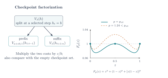
Left: the exact factorization at a checkpoint. Right: the scalar silver inequality is tight at $z=0,1/2,1$; decreasing the exponent below $p_{\mathrm{sil}}$ breaks it at the balanced split.

The correction term that closes the induction

Let $\nu \in [1/2,1)$ and set

$$\kappa ={\left(\frac{ϵ}{c-ϵ}\right)}^{\nu }.$$

The scalar condition needed by the recursion is

$$w^{\nu }+\kappa B^{\nu }\le x^{\nu }+y^{\nu }$$

whenever

$$x,y\ge a,B>0,w=x+y+B-a,wB=(c-ϵ)xy.$$

Under this condition, Lemma 3.4 proves

$$U_n(\lambda {)}^{\nu }\le a^{\nu }n+{\lambda }^{\nu }.$$

Here is the mechanism behind that bound. Call a checkpoint set tight if its cost equals $V_{\lambda }(h)$. The paper proves that $U_n(\lambda )$ is attained by a positive finite schedule for which both the empty set and a nonempty set are tight. Log-submodularity of $\Psi$ controls the tight sets:

$$\Psi (A)\Psi (B)\ge \Psi (A\cap B)\Psi (A\cup B).$$

Thus tight sets are closed under intersection and union; strictness for disjoint nonempty sets forces their intersections to be nonempty. If the empty set were not tight at a maximizing schedule, slightly decreasing a step shared by all tight sets would increase every minimizing cost, contradicting maximality. If only the empty set were tight, slightly increasing any step would produce the same contradiction.

For such an extremizing schedule, write $W=U_n(\lambda )$ and let $T=\{t_1,\dots ,t_k\}$ be a nonempty tight set. The splitting lemma in Appendix B.3 gives

$$W^{\nu }+\sum _{i=1}^k{\left(\frac{ϵb_i}{c}\right)}^{\nu }\le (\lambda +s_{k+1}{)}^{\nu }+\sum _{i=1}^k{\left(a+s_i+\frac{ϵb_i}{c}\right)}^{\nu }.$$

It also identifies each term on the right as the optimized cost of the corresponding intervening block. This is the technical bridge from the scalar condition to arbitrary checkpoint sets; its proof uses perturbations of tight schedules. The extra sum on the left records precisely the cost of the shifted prefix parameters.

Induct simultaneously on $n$ for every $\lambda \ge a$. The $k+1$ intervening blocks contain $n-k$ steps in total. Applying the induction hypothesis to them yields

$$\begin{array}{rl}{W}^{\nu }+\sum _i(ϵb_i/c{)}^{\nu }& \le a^{\nu }(n-k)+{\lambda }^{\nu }+\sum _i(a+ϵb_i/c{)}^{\nu }\\ & \le a^{\nu }n+{\lambda }^{\nu }+\sum _i(ϵb_i/c{)}^{\nu }.\end{array}$$

The second line uses $(r+s{)}^{\nu }\le r^{\nu }+s^{\nu }$ for $r,s\ge 0$ and $0<\nu <1$. Cancel the identical correction sums to obtain the claimed growth bound.

If the splitting inequality had omitted its correction term, the shifted-parameter errors would remain in the induction. This cancellation is the reason the local geometric improvement leads to a uniform lower bound for arbitrary schedules.

🏷️ The Scalar Inequality and the Silver Exponent

The limiting scalar problem

To understand the origin of the exponent, temporarily consider the ideal limiting coefficients $c=1$, $ϵ=0$. Divide the scalar relations by $w$ and put

$$u=x/w,v=y/w,p=1/\nu .$$

Then

$$u+v+uv=1+a/w\ge 1,$$

and the desired inequality is $u^{1/p}+v^{1/p}\ge 1$. If it failed, setting $X=u^{1/p}$ and $Y=v^{1/p}$ would give $Y<1-X$. Since $X^p+Y^p+X^p{Y}^p$ increases with $Y$, we would have

$$u+v+uv<X^p+(1-X{)}^p+[X(1-X){]}^p.$$

Thus the desired scalar condition follows from the silver inequality

$$z^{p_{\mathrm{sil}}}+(1-z{)}^{p_{\mathrm{sil}}}+[z(1-z){]}^{p_{\mathrm{sil}}}\le 1,0\le z\le 1.$$

At the balanced split $z=1/2$, equality requires

$$2\cdot 2^{-p}+4^{-p}=1.$$

Writing $r=2^p$ gives $r^2=2r+1$, whose positive solution is $r=1+\sqrt{2}$. Hence $p={\log }_2(1+\sqrt{2})$. The silver ratio appears because a binary split incurs a third, multiplicative term in addition to the two child contributions.

Balanced equality identifies the candidate exponent; it does not by itself prove the inequality for unbalanced splits. The paper supplies the following calculus argument.

Proof of the silver inequality

Let $p=p_{\mathrm{sil}}$, $\alpha =p-1\in (0,1/3)$, and $F(z)=z^p+(1-z{)}^p+[z(1-z){]}^p$. For $0<z<1/2$,

$$\frac{F^{\prime }(z)}{p[z(1-z){]}^{\alpha }}=\varphi (z):=(1-z{)}^{-\alpha }-z^{-\alpha }+1-2z.$$

Differentiating twice gives

$${\varphi }^{\prime \prime }(z)=\alpha (\alpha +1)\left[(1-z{)}^{-\alpha -2}-z^{-\alpha -2}\right]<0.$$

Thus ${\varphi }^{\prime }$ decreases strictly. Its endpoint behavior is ${\varphi }^{\prime }(0+)=+\infty$ and

$${\varphi }^{\prime }(1/2)=\alpha 2^{\alpha +2}-2<0.$$

The last inequality follows from $\alpha <1/3$. Consequently, $\varphi$ first increases and then decreases. Since $\varphi (0+)=-\infty$, $\varphi (1/2)=0$, and ${\varphi }^{\prime }(1/2)<0$, it is positive just left of $1/2$ and crosses zero exactly once in the interior. Therefore $F$ first decreases and then increases on $[0,1/2]$.

Its maximum on this half-interval is at an endpoint. Those values are

$$F(0)=1,F(1/2)=\frac{2}{\rho }+\frac{1}{{\rho }^2}=1.$$

Symmetry gives the other half. Equality occurs at $z=0,1/2,1$.

Perturbing the geometry

The actual construction needs $ϵ,\gamma >0$, hence $c>1$. With

$$\tau ={ϵ}^{1/p},\nu =1/p,$$

the normalized scalar constraint becomes

$$u+v+(c-ϵ)uv\ge 1,$$

and the target, including the correction term, is

$$u^{1/p}+v^{1/p}-\tau (uv{)}^{1/p}\ge 1.$$

Lemma 3.5 quantifies how much to increase $p$ to retain this inequality. For $p\in [p_{\mathrm{sil}},3/2]$, $0<c-ϵ\le 2$, and $\tau \le 1/10$, it suffices that

$$p-p_{\mathrm{sil}}\ge (c-ϵ-1{)}_{+}+6{ϵ}^{1/p},t_{+}:=\max \{t,0\}.$$

The useful slack estimate is

$$z^p+(1-z{)}^p+(c-ϵ)[z(1-z){]}^p\le 1-[p-p_{\mathrm{sil}}-(c-ϵ-1{)}_{+}]z(1-z).$$

To obtain it, differentiate with respect to $p$. The inequalities $-\log z\ge 1-z$ and $-\log (1-z)\ge z$ give a decrease of at least $z(1-z)$ per unit increase in $p$. The deviation of $c-ϵ$ from $1$ costs at most $(c-ϵ-1{)}_{+}z(1-z)$. Finally, the perturbed boundary $Y=(1-X)/(1-\tau X)$ differs from $1-X$ by at most $\tau X(1-X)/(1-\tau )$; a mean-value estimate costs at most $6\tau X(1-X)$. The displayed condition pays for both errors.

This quantitative slack is necessary near $z=0,1$, where a merely uniform continuity argument would not control the vanishing gap.

🏷️ The Finite-Horizon Bound and the Subpolynomial Loss

Choose $0<\eta \le 1/10$ and set

$$p=p_{\mathrm{sil}}+\eta ,\gamma =\eta /4,ϵ=(\eta /16{)}^p.$$

Then ${ϵ}^{1/p}=\eta /16$ and $c\le 1+\eta /3$. In particular,

$$(c-ϵ-1{)}_{+}+6{ϵ}^{1/p}\le \frac{\eta }{3}+\frac{3\eta }{8}=\frac{17\eta }{24}<\eta .$$

The scalar hypothesis holds, so the recursive bound is available with $\nu =1/p$. Now choose $\lambda =a{n}^p$. It gives

$$U_n(\lambda {)}^{\nu }\le a^{\nu }n+{\lambda }^{\nu }=2a^{\nu }n,U_n(\lambda )\le 2^{p}a{n}^p.$$

Substitution into the error estimate yields

$${\mathcal{R}}_n(h)\ge \frac{1}{2^{2p+1}a}{n}^{-p}.$$

The choice of $\lambda$ matters: its numerator contributes $n^p$, compensating for one of the two powers of the cost in the denominator. Fixing $\lambda$ would lose this sharp exponent.

For every fixed $p>p_{\mathrm{sil}}$, this already rules out rate $O(n^{-q})$ for any $q>p$, uniformly over all schedules. To approach $p_{\mathrm{sil}}$ as the horizon grows, we must track the prefactor $1/a$.

The explicit turning constant contains an exponent $R/\gamma =O(1/\eta )$ and a base whose logarithm is $O(\log (1/\eta ))$. Since $a$ can be chosen as

$$a=\max \{2,2C_0/c,2B_0+2\},$$

the paper obtains

$$\log a=O\left({\eta }^{-1}\log (1/\eta )\right).$$

Consequently,

$${\mathcal{R}}_n(h)\ge n^{-p_{\mathrm{sil}}}\exp \left[-\eta \log n-O\left({\eta }^{-1}\log (1/\eta )\right)\right].$$

There are two costs: using exponent $p_{\mathrm{sil}}+\eta$ contributes $\eta \log n$, and making the gradient arc nearly ideal enlarges the construction constants. Taking

$$\eta =\sqrt{\frac{\log \log n}{\log n}}$$

balances them at order $\sqrt{\log n\log \log n}$. This proves Theorem 1.1.

The word “almost” in the title refers to this remaining subpolynomial factor. It is a quantitative loss from the construction, while optimality of the polynomial exponent follows rigorously.

🏷️ Anytime Schedules and Record-Time Obstructions

Total step size and the largest step

For a fixed infinite schedule, define

$$S_n=\sum _{t=1}^n{h}_t,M_n=\underset{1\le t\le n}{\max }{h}_t,r_n={\mathcal{R}}_n(H_n).$$

A record time is an index with $h_n=M_n$. An unbounded schedule has infinitely many strict record times, where $h_n>M_{n-1}$. These horizons expose a long step before later steps can compensate for it.

If the schedule is bounded, then $S_n=O(n)$, and the no-checkpoint bound

$$r_n\ge \frac{1}{4(1+S_n)}$$

already gives a lower bound of order $n^{-1}$, stronger than required. Thus the interesting case has infinitely many growing records.

Fix $p>p_{\mathrm{sil}}$ close to $p_{\mathrm{sil}}$ and $\nu =1/p$. Lemma 4.1 establishes the following restriction at record times with $M_n\ge B_0$ and sufficiently small $r_n$:

$$S_n\le C_{p}n{M}_n^{1-\nu }.$$

This improves the elementary estimate $S_n\le n{M}_n$. A schedule with small record-time error cannot have arbitrarily many large steps.

Counting steps above a threshold

The proof uses the same checkpoint costs. At a record time, put $M=h_n$, $\xi =H_{n-1}$, $\Lambda =a+ϵM/c$, and $V=V_{\Lambda }(\xi )$. Append the final step $M$ to a minimizing checkpoint set for this prefix. Lemma 2.2 gives

$$r_n\ge \frac{M^2}{4c^2{V}^2},V\ge \frac{M}{2c\sqrt{r_n}}.$$

When $r_n$ is sufficiently small, $V\ge 2M$. This lower bound on prefix cost prevents too many large steps from making that cost small.

For $0<u\le M$, define the threshold count

$$N_{\xi }(u)=\#\{t<n:h_t>u\}.$$

If there are $k$ such steps, select all of them and optimize checkpoints within the blocks between them. Apply the finite-horizon cost bound to each block. The factorization and $1+z\le e^z$ yield

$$\frac{cV}{ϵM}\le {ϵ}^k\exp \left(\frac{(ac/ϵ{)}^{\nu }}{\nu }n{u}^{-\nu }\right).$$

The optimized cost $V$ is at most the cost of this chosen set. Each selected large step contributes a factor $ϵ$, whereas the remaining block contributions are controlled by their total number of iterations. Since $V\ge 2M$, the left side exceeds $1$. Taking logarithms therefore bounds

$$N_{\xi }(u)\le \frac{(ac/ϵ{)}^{\nu }}{\nu \log (1/ϵ)}n{u}^{-\nu }.$$

These selected threshold steps need not exceed $B_0$: this part uses algebraic checkpoint costs, not a new invocation of the hard-function lemma at those steps. The earlier invocation with the final record step uses admissible checkpoints.

Integrate the threshold count, using the exact layer-cake identity

$$\sum _{t<n}{h}_t={\int }_0^M{N}_{\xi }(u)du.$$

Because $\nu <1$, the integral of $u^{-\nu }$ is finite and equals $M^{1-\nu }/(1-\nu )$. Thus

$$\sum _{t<n}{h}_t\le K_{p}n{M}^{1-\nu }.$$

To include the final step, compare $V\ge 2M$ with the cost growth bound:

$$2^{\nu }{M}^{\nu }\le V^{\nu }\le a^{\nu }(n-1)+(a+ϵM/c{)}^{\nu }\le a^{\nu }n+(ϵM/c{)}^{\nu }.$$

It follows that $M^{\nu }\le K_{p}n$, hence $M\le K_{p}n{M}^{1-\nu }$. This proves the record-time sum estimate.

Deriving the exponent $2p/(1+p)$

At a record time, selecting only the final step gives

$$r_n\ge \frac{1}{4}{\left[\frac{M_n}{c(a+S_{n-1})+ϵM_n}\right]}^2.$$

For sufficiently small $r_n$, rearrange this inequality and absorb the $ϵM_n$ term to obtain

$$M_n\le K_p{S}_n\sqrt{r_n}.$$

The no-checkpoint bound also implies $S_n\ge 1/(8r_n)$ when $r_n\le 1/8$. Combining these two estimates with the record-time sum bound gives

$$S_n\le C_{p}n(K_p{S}_n\sqrt{r_n}{)}^{1-\nu },S_n^{\nu }\le K_{p}n{r}_n^{(1-\nu )/2}.$$

Insert $S_n\ge 1/(8r_n)$ and rearrange:

$$1\le K_{p}n{r}_n^{(1+\nu )/2},r_n\ge c_p{n}^{-2/(1+\nu )}=c_p{n}^{-2p/(1+p)}.$$

This calculation explains the anytime exponent. Small error requires a large total step sum, yet small error immediately after a record constrains the record’s size relative to that sum. The checkpoint recursion bounds how densely large steps can occur. Together these requirements force the smaller exponent.

The constants satisfy

$$\log (1/c_p)+\log (1/r_{0,p})=O\left((p-p_{\mathrm{sil}}{)}^{-1}\log \frac{1}{p-p_{\mathrm{sil}}}\right),$$

where $r_{0,p}$ is the small-error threshold. At each sufficiently large strict record time, take $p-p_{\mathrm{sil}}={\delta }_n$. Since

$$\frac{2p}{1+p}=p_{\mathrm{any}}+O({\delta }_n),$$

the same balance of constants yields Theorem 1.2. If the record is below the required threshold or its error exceeds $r_{0,p}$, the elementary lower bounds are already stronger. Infinitely many strict records remain, completing the anytime argument.

The choice of $p$ and the hard objective can vary with $n$ because each $r_n$ is a separate worst-case supremum. The infinite schedule itself remains fixed throughout.

🏷️ Consequences, Limitations, and Further Questions

The two lower bounds settle the optimal polynomial exponents for the stated algorithm class. In the finite-horizon problem,

$$n^{-p_{\mathrm{sil}}-o(1)}\le r_n^{\ast }\le C{n}^{-p_{\mathrm{sil}}},$$

so the asymptotic logarithmic exponent is $p_{\mathrm{sil}}$. For anytime schedules, an upper bound with exponent $p_{\mathrm{any}}$ holds at every horizon, while the lower bound obstructs every larger fixed exponent along infinitely many horizons.

The construction makes three features of the result particularly transparent. Smoothness permits gradients to rotate, and flat zero regions permit sequential activation. Predetermined steps allow the adversary to arrange those regions around the entire schedule. Finally, the global recursion must preserve enough quantitative information to pay for every shifted local parameter; the correction sum is essential to this accounting.

Two questions remain open in the version discussed here (Ye & Liu, 2026). One is extending matching lower bounds to schedules with negative steps. Nonnegativity enters the coordinate monotonicity, zero-set invariants, and positive checkpoint costs, so this would require additional arguments. The other is reducing or removing the subpolynomial loss and obtaining a sharper comparison with the upper bounds. The paper mentions preliminary work with logarithmic spirals in gradient space; it does not prove such an improvement in this version.

Source map for the detailed arguments

This exposition includes the local construction, smoothness and loss calculations, the recursive cancellation, the scalar proof, and the anytime exponent derivation. The following locations supply the longer technical verifications used above:

Paper location	Role in the proof
Lemmas 3.1–3.2; Appendix A.1–A.2	Backward projection invariants, turning bound, finite envelope, and zero sets
Lemma 2.2; Appendix A.3	Sequential activation and the globally smooth coordinate chain
Lemma 3.3; Appendix B.1–B.2	Admissibility of minimizing checkpoints and exact factorization
Lemma 3.4; Appendix B.3	Attainment of extremal schedules, log-submodularity, and the splitting inequality
Lemma 3.5; Appendix B.4–B.5	Silver inequality, perturbative slack, and explicit constant growth
Lemma 4.1; Appendix C	Threshold counting at records and the final anytime argument

Links

• on Q-D recursive Runge-Kutta methods: both topics design sequences of step coefficients using information across a whole block. The Runge–Kutta post concerns accuracy conditions for ODE solvers; here the coefficients control worst-case optimization error.
• on new bounds for the real Grothendieck constant: a related example of optimization upper bounds paired with universal obstructions. The role of $1+\sqrt{2}$ in that post comes from a different analytic mechanism; here it comes from the balanced checkpoint split.

📚 References

🐻  Altschuler, J.M. & Parrilo, P.A. 2025. Acceleration by stepsize hedging: Silver Stepsize Schedule for smooth convex optimization. Mathematical Programming 213(1–2), 1105–1118.

🐻  Jung, M., Cho, H. & Yun, C. 2026. Stronger Lower Bounds for (Non-)Anytime Acceleration of Gradient Descent.

🐻  Moreau, J.-J. 1965. Proximité et dualité dans un espace hilbertien. Bulletin de la Société Mathématique de France 93, 273–299.

🐻  Ye, Y. & Liu, K. 2026. Silver Rate Is (Almost) Optimal for Gradient Descent.

🐻  Zhang, Z., Lee, J.D., Du, S.S. & Chen, Y. 2025. Anytime Acceleration of Gradient Descent. In Proceedings of Thirty Eighth Conference on Learning Theory, pp. 5991–6013. Proceedings of Machine Learning Research, PMLR.