on new bounds for the real Grothendieck constant

Overview

Li, Saha, Xue, Chaudhuri, Klivans, Kothari, and Meka state new lower and upper bounds for the real Grothendieck constant $K_G$ (Li et al., 2026); complete proofs appear in the companion paper by Saha and collaborators (Saha et al., 2026):

$$\begin{array}{rl}\frac{6\pi }{11}& \le K_G\le 1.7818666069360661,\\ K_G& <\frac{\pi }{2\log (1+\sqrt{2})}-3.4737\cdot 10^{-4}.\end{array}$$

The upper bound comes from a limiting cubic–quintic Krivine rounding scheme. The lower bound comes from a universal affine obstruction

$$b_3\ge 2b_1-\frac{11}{6}$$

on the first and third coefficients of every Krivine correlation function. This is the first lower-bound mechanism of its kind: it limits all asymptotically optimal rounding schemes instead of constructing one explicit hard matrix.

🏷️ The Grothendieck Optimization Problem

Let $A=(a_{ij})\in {\mathbb{R}}^{m\times n}$. Define the discrete bilinear optimum

$$\mathrm{OPT}(A)=\underset{\begin{array}{c}{\epsilon }_i\in \{-1,1\}\\ {\delta }_j\in \{-1,1\}\end{array}}{\max }\left|\sum _{i=1}^m\sum _{j=1}^n{a}_{ij}{\epsilon }_i{\delta }_j\right|.$$

The variables label the rows and columns by signs. This problem contains cut-type optimization problems and is NP-hard in general.

Replace every sign by a unit vector and every product by an inner product:

$$\mathrm{SDP}(A)=\underset{\begin{array}{c}\Vert u_i\Vert =1\\ \Vert v_j\Vert =1\end{array}}{\sup }\left|\sum _{i=1}^m\sum _{j=1}^n{a}_{ij}⟨u_i,v_j⟩\right|.$$

It is enough to take the vectors in ${\mathbb{R}}^{m+n}$, because the Gram matrix of $m+n$ vectors has rank at most $m+n$. Equivalently, the variables are entries of a positive-semidefinite Gram matrix with diagonal equal to $1$, so this is a semidefinite program.

Every sign assignment is a one-dimensional unit-vector assignment. Hence

$$\mathrm{OPT}(A)\le \mathrm{SDP}(A).$$

The absolute value is equivalent to the unsigned maximum: flipping every row sign reverses the bilinear form. This convention therefore agrees with the standard formulation of Grothendieck’s inequality.

Grothendieck’s inequality asserts that the reverse comparison loses only a universal constant (Grothendieck, 1953).

Real Grothendieck inequality

There is a finite constant $K$, independent of $m,n$, and $A$, such that

$$\mathrm{SDP}(A)\le K\mathrm{OPT}(A)$$

for every real matrix $A$. The real Grothendieck constant is

$$K_G=\underset{A\ne 0}{\sup }\frac{\mathrm{SDP}(A)}{\mathrm{OPT}(A)}.$$

Thus $K_G$ is the worst-case integrality gap of this canonical SDP relaxation. An upper bound on $K_G$ is a rounding theorem: it gives a randomized procedure that turns every vector solution into signs while retaining a definite fraction of its value. A lower bound shows that no rounding procedure can close the relaxation gap beyond a certain point.

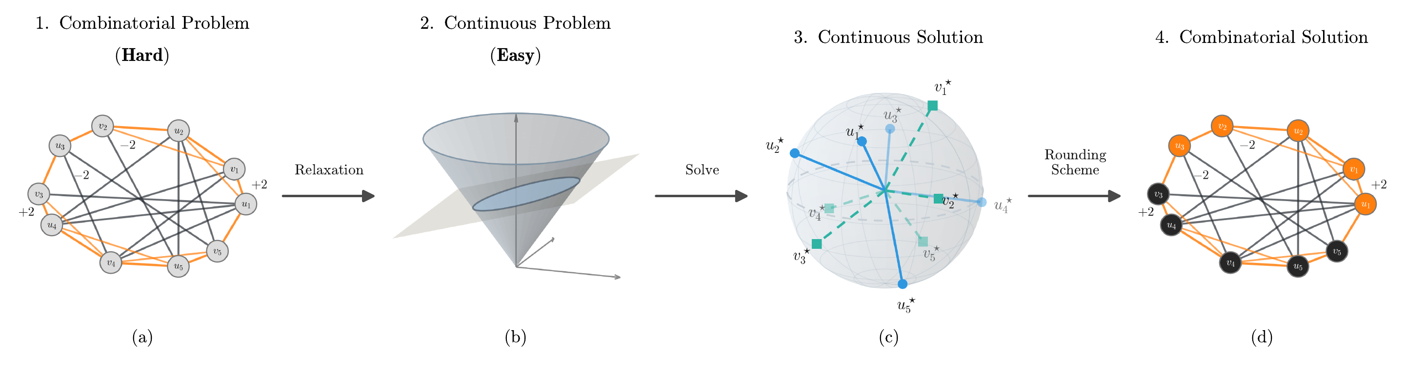
The figure displays the relaxation-and-rounding pipeline used in the paper. The middle vector solution is efficiently accessible; the mathematical problem is to discretize it without losing too much of the objective.

Historical Scale of the Gap

Krivine proved the classical upper bound

$$K_G\le K_{\mathrm{Kr}}:=\frac{\pi }{2\log (1+\sqrt{2})}=1.7822139781913693\dots$$

(Krivine, 1977). He conjectured equality. Braverman, Makarychev, Makarychev, and Naor later proved that the inequality is strict (Braverman et al., 2013). Naor and Regev then showed that mixed Krivine schemes become optimal as their dimension grows (Naor & Regev, 2014).

Before the two 2026 papers, the lower side was approximately

$$K_G\ge 1.6769566742,$$

coming from high-dimensional constructions of Davie and Reeds and only minutely improved in recent work (Saha et al., 2026). The new interval

$$1.7135959928671598\dots \le K_G\le 1.7818666069360661\dots$$

determines the previously unknown tenths digit: every admissible value begins with $1.7$.

🏷️ Correlated Gaussians and Hermite Expansions

The rounding analysis converts geometry on the sphere into harmonic analysis on Gaussian space.

Correlated Gaussian Pairs

For $t\in (-1,1)$, let $X,Z\sim N(0,I_d)$ be independent and set

$$Y_t=tX+\sqrt{1-t^2}Z.$$

Then $X$ and $Y_t$ are standard Gaussian vectors with

$$\mathbb{E}[X_i(Y_t{)}_j]=t{\delta }_{ij}.$$

The parameter $t$ will later be the inner product of two preprocessed SDP vectors.

For one-dimensional signs, the Gaussian quadrant identity gives

$$\mathbb{E}[\mathrm{sgn}(X)\mathrm{sgn}(Y_t)]=\frac{2}{\pi }\arcsin t.$$

This identity is the origin of the normalization used throughout the paper.

Orthonormal Hermite Basis

Let ${\gamma }_d$ be standard Gaussian measure on ${\mathbb{R}}^d$. The first orthonormal probabilists’ Hermite polynomials are

$${\psi }_0(s)=1,{\psi }_1(s)=s,{\psi }_2(s)=\frac{s^2-1}{\sqrt{2}},{\psi }_3(s)=\frac{s^3-3s}{\sqrt{6}}.$$

For a multi-index $\alpha \in {\mathbb{N}}^d$, define

$${\psi }_{\alpha }(x)=\prod _{i=1}^d{\psi }_{{\alpha }_i}(x_i),|\alpha |=\sum _{i=1}^d{\alpha }_i.$$

These functions form an orthonormal basis of $L^2({\gamma }_d)$. Write $P_{q}F$ for the projection of $F$ onto total Hermite degree $q$.

Mehler’s identity states that

$$\mathbb{E}[F(X)G(Y_t)]=\sum _{q=0}^{\infty }{t}^q⟨P_{q}F,P_{q}G{⟩}_{L^2({\gamma }_d)}.$$

In particular,

$$\mathbb{E}[{\psi }_{\alpha }(X){\psi }_{\beta }(Y_t)]=1_{\{\alpha =\beta \}}{t}^{|\alpha |}.$$

A pure degree-$q$ Hermite component therefore remembers correlation through the power $t^q$. This simple fact drives both the cubic–quintic upper bound and the coefficient obstruction in the lower bound.

If $F$ is odd, then $P_{q}F=0$ for even $q$. Thus correlations of odd partitions have odd power-series expansions.

First-degree projection

For $F\in L^2({\gamma }_d)$,

$$P_{1}F(x)=⟨c_F,x⟩,c_F=\mathbb{E}[F(X)X].$$

If $|F|\le 1$, then

$$\Vert P_{1}F\Vert =\underset{\Vert e\Vert =1}{\sup }|\mathbb{E}[F(X)⟨e,X⟩]|\le \mathbb{E}|Z|=\nu ,\nu :=\sqrt{\frac{2}{\pi }}.$$

The Gaussian comparison viewpoint is complementary to on Slepian’s lemma and Gaussian comparison: there the covariance orders suprema, whereas here it parametrizes the exact correlation profile of a rounding partition.

🏷️ Krivine Schemes and the Inverse Majorant

A $d$-dimensional Krivine scheme is a pair of odd measurable partitions

$$f,g:{\mathbb{R}}^d⟶\{-1,1\}.$$

Given a correlated Gaussian pair $(X,Y_t)$, define its arcsine-normalized correlation function

$$H_{f,g}(t):=\frac{\pi }{2}\mathbb{E}[f(X)g(Y_t)].$$

Hermite expansion gives

$$H_{f,g}(t)=\frac{\pi }{2}\sum _{\begin{array}{c}q\ge 1\\ q\mathrm{odd}\end{array}}⟨P_{q}f,P_{q}g⟩t^q.$$

Write

$$H(t)=b_{1}t+b_3{t}^3+b_5{t}^5+\cdots .$$

If $b_1=H^{\prime }(0)\ne 0$, the holomorphic inverse function theorem gives a local odd inverse

$$H^{-1}(z)=\sum _{\begin{array}{c}r\ge 1\\ r\mathrm{odd}\end{array}}{a}_r{z}^r.$$

Its absolute-coefficient majorant is

$$M_H(s):=\sum _{\begin{array}{c}r\ge 1\\ r\mathrm{odd}\end{array}}|a_r|s^r.$$

Krivine inverse-majorant criterion

If

$$M_H(\gamma )\le 1,$$

with the inverse holomorphic on a neighborhood of the closed disk of radius $\gamma$, then

$$K_G\le \frac{\pi }{2\gamma }.$$

The theorem is not merely a formal power-series trick. It constructs the preprocessing map used by the rounding algorithm.

Proof: Tensor Preprocessing and Gaussian Projection

Fix $0<{\gamma }^{\prime }<\gamma$, so

$$m_{{\gamma }^{\prime }}:=\sum _r|a_r|({\gamma }^{\prime }{)}^r<1.$$

If the original unit vectors lie in a Hilbert space $\mathcal{H}$, work in

$$\mathcal{K}=\left(\underset{r\ge 1}{⨁}{\mathcal{H}}^{\otimes r}\right)\oplus \mathbb{R}{e}_L\oplus \mathbb{R}{e}_R.$$

For unit $x,y$, set

$$I(x)=\underset{r\ge 1}{⨁}\sqrt{|a_r|}({\gamma }^{\prime }{)}^{r/2}{x}^{\otimes r}\oplus \sqrt{1-m_{{\gamma }^{\prime }}}{e}_L\oplus 0$$

and

$$J(y)=\underset{r\ge 1}{⨁}\mathrm{sgn}(a_r)\sqrt{|a_r|}({\gamma }^{\prime }{)}^{r/2}{y}^{\otimes r}\oplus 0\oplus \sqrt{1-m_{{\gamma }^{\prime }}}{e}_R.$$

The unused orthogonal directions make both new vectors unit. Since

$$⟨x^{\otimes r},y^{\otimes r}⟩=⟨x,y{⟩}^r,$$

one has

$$⟨I(x),J(y)⟩=H^{-1}({\gamma }^{\prime }⟨x,y⟩).$$

Because only the finitely many vectors $I(u_i)$ and $J(v_j)$ are used, it is enough to define a Gaussian map on their finite-dimensional span. Apply such a random map $\Gamma :\mathcal{K}\to {\mathbb{R}}^d$ and round by

$${\epsilon }_i=f(\Gamma I(u_i)),{\delta }_j=g(\Gamma J(v_j)).$$

Gaussian rotation invariance gives

$$\mathbb{E}[{\epsilon }_i{\delta }_j]=\frac{2}{\pi }H(⟨I(u_i),J(v_j)⟩)=\frac{2{\gamma }^{\prime }}{\pi }⟨u_i,v_j⟩.$$

Therefore

$$\mathrm{OPT}(A)\ge \frac{2{\gamma }^{\prime }}{\pi }\mathrm{SDP}(A).$$

Letting ${\gamma }^{\prime }\uparrow \gamma$ proves the claim.

Hyperplane Rounding

Take $f=g=\mathrm{sgn}$ on $\mathbb{R}$. Then

$$H(t)=\arcsin t,H^{-1}(z)=\sin z.$$

The majorant of $\sin z$ is

$$M_H(s)=\sum _{q\ge 0}\frac{s^{2q+1}}{(2q+1)!}=\sinh s.$$

The equation $M_H(\gamma )=1$ has solution

$$\gamma =\mathrm{arsinh}(1)=\log (1+\sqrt{2}).$$

The inverse-majorant criterion recovers Krivine’s classical bound.

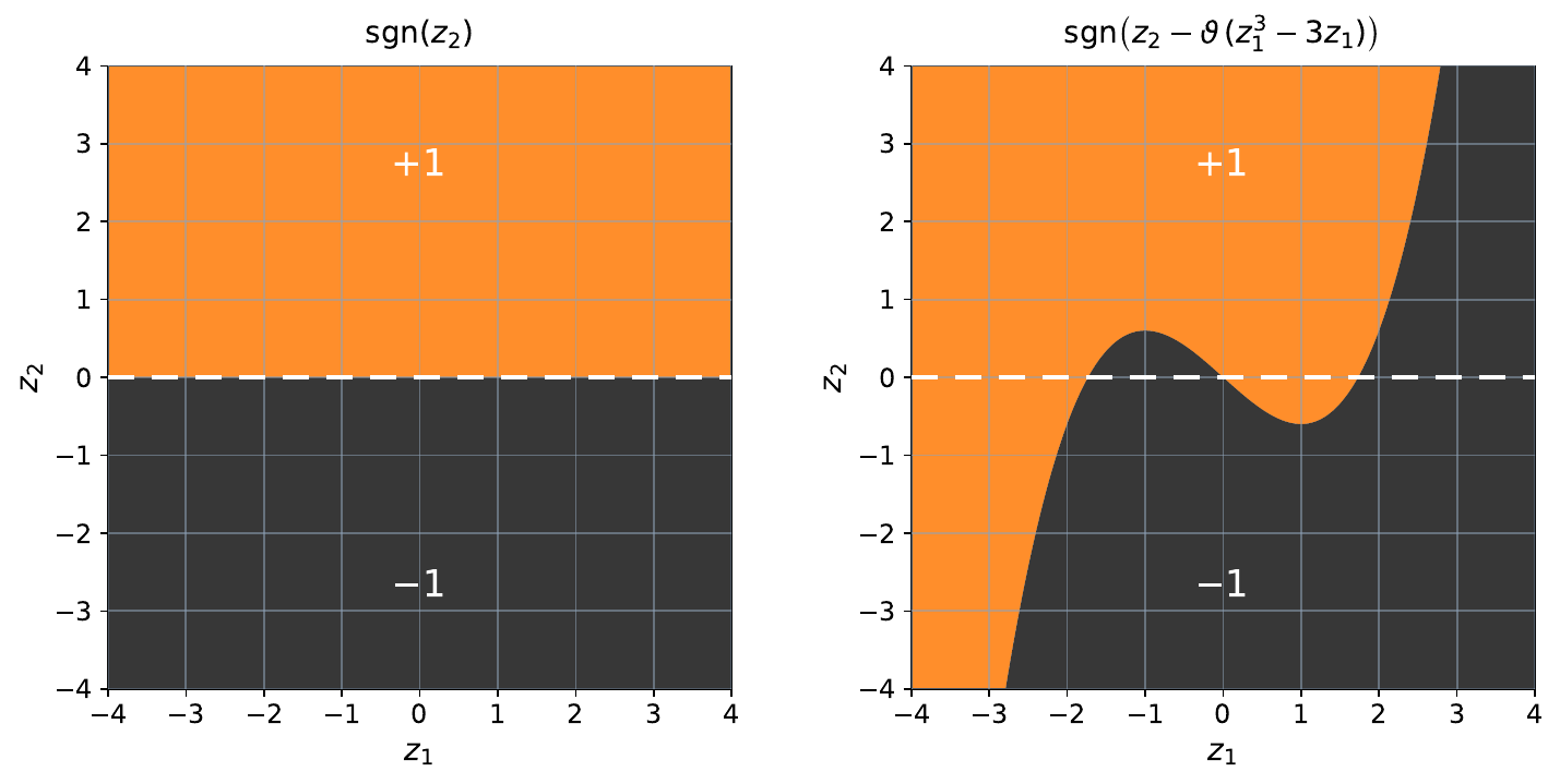
The left partition is a half-space and produces the arcsine profile. The curved boundary on the right is a cubic threshold of the type used below; its displayed coefficient absorbs the factor $1/\sqrt{6}$ in the normalized polynomial ${\psi }_3$.

🏷️ Limiting and Mixed Krivine Schemes

The upper bound does not optimize a fixed low-dimensional partition. It introduces a compact analytic language for limits of ordinary schemes whose dimensions tend to infinity.

Allowable Correlation Maps

An odd function $\rho :(-1,1)\to \mathbb{R}$ is allowable when

$$\rho (t)=\sum _{\begin{array}{c}q\ge 1\\ q\mathrm{odd}\end{array}}{c}_q{t}^q,\sum _q|c_q|\le 1.$$

A limiting $d$-dimensional scheme consists of measurable odd sign functions $f,g:{\mathbb{R}}^d\to \{-1,1\}$ whose discontinuity sets have Gaussian measure zero, together with allowable maps ${\rho }_1,\dots ,{\rho }_d$. Its Gaussian coordinates satisfy

$$\mathbb{E}[X_i{Y}_j]={\delta }_{ij}{\rho }_i(t)$$

instead of the classical restriction ${\rho }_i(t)=t$.

Allowability is exactly what is needed for a Hilbert-space realization. If $s={\sum }_q|c_q|$, define odd, unit-$L^2$ functions

$$p(x)=\sum _q\sqrt{|c_q|}{\psi }_q(x_1)+\sqrt{1-s}{x}_2$$

and

$$q(y)=\sum _q\mathrm{sgn}(c_q)\sqrt{|c_q|}{\psi }_q(y_1)+\sqrt{1-s}{y}_3.$$

For coordinatewise $t$-correlated Gaussian triples $U,V$,

$$\mathbb{E}[p(U)q(V)]=\rho (t).$$

Central-Limit Realization

The basic example is the correlation $t^3$. Let

$$U_N=\frac{1}{\sqrt{N}}\sum _{j=1}^N{\psi }_3(X_j),V_N=\frac{1}{\sqrt{N}}\sum _{j=1}^N{\psi }_3(Y_j),$$

where the pairs $(X_j,Y_j)$ are independent and $t$-correlated. Then

$$\mathbb{E}[U_N{V}_N]=t^3.$$

The multivariate central limit theorem sends $(U_N,V_N)$ to a correlated Gaussian pair with correlation $t^3$. Applying the same construction to every allowable coordinate produces ordinary, increasingly high-dimensional Krivine schemes whose correlation functions converge pointwise to the limiting one.

The proof needs two analytic upgrades.

1. Hermite expansions make every finite correlation function holomorphic on the unit disk and uniformly bounded there by $\pi /2$. Vitali’s theorem upgrades pointwise convergence on $(-1,1)$ to locally uniform convergence on the disk.

2. Local uniform convergence of $H_N\to H$ does not by itself control every coefficient of $H_N^{-1}$. Rouché’s theorem preserves the inverse branch on a slightly smaller disk, fixed inverse coefficients converge by Cauchy’s formula, and a Cauchy estimate on a larger disk controls the remaining tail uniformly. A strict certificate $M_H(\gamma )<1$ therefore transfers to all sufficiently large finite-dimensional approximations.

Finite-dimensional status of limiting schemes

The fixed-dimensional limiting model is an analysis device. The actual algorithms are ordinary finite-dimensional Gaussian schemes. The transfer theorem proves existence for all sufficiently large dimensions, but the paper does not optimize or display the first usable finite dimension.

Mixtures

A mixed scheme samples one pair $(f,g)$ from a probability distribution and uses that same global pair for every row and column. Its averaged correlation function is

$$H_{\mu }(t)={\mathbb{E}}_{(f,g)\sim \mu }{H}_{f,g}(t).$$

The global sampling is essential: independently choosing a scheme for every matrix entry would not define consistent signs.

Mixtures matter twice. They were used to disprove equality in Krivine’s classical bound, and the Naor–Regev optimality theorem says that mixed schemes in increasing dimension approach the true constant (Naor & Regev, 2014). Most importantly for the new lower bound, any affine inequality in the coefficients of $H$ is automatically preserved by averaging and coefficientwise limits.

🏷️ Main Bounds

New interval for the real Grothendieck constant

The real Grothendieck constant satisfies

$$\frac{6\pi }{11}\le K_G\le \mathrm{1.7818666069360661.}$$

The upper inequality is obtained from an explicit limiting Krivine scheme whose inverse majorant is controlled by a finite interval certificate. The lower inequality follows from a universal relation between the first and third Hermite coefficients of every Krivine scheme, followed by the asymptotic optimality of mixed schemes.

🏷️ The Cubic–Quintic Upper Bound

The Explicit Limiting Scheme

Take the exact decimal parameters

$$\eta =0.136419125,s_3=0.34101124,s_5=0.05276111,$$

and set

$$V=1+s_3^2+s_5^2,\vartheta =\frac{\eta }{\sqrt{V}}.$$

The first Gaussian coordinate has the allowable correlation map

$$\rho (t)=\frac{t-s_3^2{t}^3+s_5^2{t}^5}{V},$$

while the second retains correlation $t$. The signs are separated by opposite cubic boundaries:

$$f(w,x)=\mathrm{sgn}\left(w+\vartheta {\psi }_3(x)\right),g(w,x)=\mathrm{sgn}\left(w-\vartheta {\psi }_3(x)\right).$$

Equivalently, $g(w,x)=f(w,-x)$. The negative cubic term in $\rho$ is an anti-aligned third-chaos reservoir; the positive quintic term is an aligned fifth-chaos reservoir.

The parameter choice is easier to understand from the first coefficients of the inverse. If

$$H(t)=b_{1}t+b_3{t}^3+b_5{t}^5+O(t^7)$$

and

$$H^{-1}(z)=a_{1}z+a_3{z}^3+a_5{z}^5+O(z^7),$$

then formal composition gives

$$a_1=\frac{1}{b_1},a_3=-\frac{b_3}{b_1^4},a_5=\frac{3b_3^2-b_1{b}_5}{b_1^7}.$$

The construction nearly annihilates $b_3$ and $b_5$, and hence removes the first two nonlinear obstructions in the inverse majorant, while keeping $b_1$ large.

Exact Coefficient Reduction

Let

$$A_{a,b}:=\mathbb{E}\left[f(W,X){\psi }_a(W){\psi }_b(X)\right],$$

for independent standard Gaussians $W,X$. Mehler’s identity and $g(w,x)=f(w,-x)$ give the exact expansion

$$H(t)=\frac{\pi }{2}\sum _{a,b\ge 0}{A}_{a,b}^2\rho (t{)}^a(-t{)}^b.$$

Consequently,

$$b_m=\frac{\pi }{2}\sum _{\begin{array}{c}a,b\ge 0\\ a+b\le m\end{array}}(-1{)}^b{A}_{a,b}^2[t^{m-b}]\rho (t{)}^a.$$

Parity forces every even $b_m$ to vanish.

The apparent two-dimensional integration reduces to one dimension. Define

$$q_a(u):=\mathbb{E}\left[\mathrm{sgn}(Z+u){\psi }_a(Z)\right].$$

Conditioning on $X$ yields

$$A_{a,b}=\mathbb{E}\left[{\psi }_b(X)q_a\left(\vartheta {\psi }_3(X)\right)\right].$$

With $\phi (u)=(2\pi {)}^{-1/2}{e}^{-u^2/2}$,

$$q_0(u)=\mathrm{erf}\left(\frac{u}{\sqrt{2}}\right),q_a(u)=\frac{2\phi (u)}{\sqrt{a}}{\psi }_{a-1}(-u)(a\ge 1).$$

Thus each coefficient is obtained from finitely many coefficient extractions and rigorously enclosed one-dimensional Gaussian integrals.

A Near-Linearity Certificate

Define the nonlinear coefficient mass

$${\Delta }_H:=\sum _{\begin{array}{c}m\ge 3\\ m\mathrm{odd}\end{array}}|b_m|.$$

The paper’s useful analytic simplification is that one need not directly invert hundreds of interval-valued coefficients.

Inverse certificate from near-linearity

If $b_1>0$ and

$$\gamma +{\Delta }_H<b_1,$$

then the local inverse extends holomorphically beyond the disk of radius $\gamma$ and

$$M_H(\gamma )\le \frac{\gamma +{\Delta }_H}{b_1}<1.$$

To see the mechanism, write $H(t)=b_{1}t+E(t)$ and replace $E$ by its positive-coefficient majorant

$$E_{\mathrm{maj}}(u)=\sum _{m\ge 3}|b_m|u^m.$$

There is a unique nonnegative formal series $V$ satisfying

$$b_{1}V(z)=z+E_{\mathrm{maj}}(V(z)).$$

Coefficient induction in $b_1{H}^{-1}(z)=z-E(H^{-1}(z))$ gives

$$|[z^n]H^{-1}(z)|\le [z^n]V(z).$$

For $R>\gamma$ sufficiently close to $\gamma$, the iteration

$$V_{k+1}(z)=\frac{z+E_{\mathrm{maj}}(V_k(z))}{b_1},V_0=0,$$

stays below $(R+{\Delta }_H)/b_1<1$ at $z=R$. Monotone convergence therefore proves both holomorphic control and the displayed majorant estimate.

Head, Tail, and the Final Inequality

The finite coefficient head and an analytic Sobolev-type tail are certified separately. Let

$$D=t\frac{d}{dt}.$$

Parseval on the unit circle $\mathbb{T}$ gives

$$\Vert D^{3}H{\Vert }_{L^2(\mathbb{T})}^2=\sum _{\begin{array}{c}m\ge 1\\ m\mathrm{odd}\end{array}}{m}^6|b_m{|}^2.$$

Cauchy–Schwarz and a decreasing-integral estimate imply, for odd $N$,

$$\sum _{\begin{array}{c}m>N\\ m\mathrm{odd}\end{array}}|b_m|\le \Vert D^{3}H{\Vert }_{L^2(\mathbb{T})}{\left(\sum _{\begin{array}{c}m>N\\ m\mathrm{odd}\end{array}}{m}^{-6}\right)}^{1/2}\le \frac{\Vert D^{3}H{\Vert }_{L^2(\mathbb{T})}}{\sqrt{10N^5}}.$$

At $N=251$, Arb interval arithmetic (Johansson, 2017) certifies

$$b_1\ge 0.881573822049,$$ $$\sum _{\begin{array}{c}3\le m\le 251\\ m\mathrm{odd}\end{array}}|b_m|\le 1.1328860\cdot 10^{-5},$$

and

$$\Vert D^{3}H{\Vert }_{L^2(\mathbb{T})}<\mathrm{14.443.}$$

It follows that

$${\Delta }_H<1.1328860\cdot 10^{-5}+\frac{14.443}{\sqrt{10\cdot 251^5}}<1.5904724\cdot 10^{-5}.$$

For

$$\gamma =0.881545409,$$

the decisive strict margin is

$$\gamma +{\Delta }_H<0.881561313724<0.881573822049\le b_1.$$

The near-linearity certificate, finite-dimensional transfer, and tensor preprocessing now give

$$K_G\le \frac{\pi }{2\gamma }\le \mathrm{1.7818666069360661.}$$

Analytic cost of the numerical gain

The gain over Krivine is only $3.4737\cdot 10^{-4}$, but the proof must establish a strict inequality for an infinite inverse series, show that its limiting Gaussian construction is approximated by honest finite-dimensional schemes, and enclose all numerical error. The small final change in $K_G$ hides a substantial analytic and certification problem.

🏷️ The Universal Affine Obstruction

The lower bound reverses the usual direction of attack. Instead of exhibiting a matrix $A$ with a large integrality gap, it proves that every Krivine correlation profile lies in an affine strip. The optimality theorem for mixed high-dimensional schemes then converts that universal rounding obstruction into a lower bound on $K_G$.

Coefficients and Agreement–Disagreement Variables

For arbitrary odd signs $f,g:{\mathbb{R}}^d\to \{-1,1\}$,

$$b_1=\frac{\pi }{2}⟨P_{1}f,P_{1}g⟩,b_3=\frac{\pi }{2}⟨P_{3}f,P_{3}g⟩.$$

Set

$$h=\frac{f+g}{2},k=\frac{f-g}{2}.$$

Then $h,k\in \{-1,0,1\}$, $hk=0$, and

$$h^2+k^2=1.$$

The function $h$ records agreement and $k$ disagreement. Writing $u=P_{1}h$ and $v=P_{1}k$, one obtains

$$⟨P_{1}f,P_{1}g⟩=\Vert u{\Vert }^2-\Vert v{\Vert }^2,$$ $$\Vert P_{1}f\Vert \Vert P_{1}g\Vert \le \Vert u{\Vert }^2+\Vert v{\Vert }^2,$$

and

$$⟨P_{3}f,P_{3}g⟩=\Vert P_{3}h{\Vert }^2-\Vert P_{3}k{\Vert }^2.$$

It is therefore enough to prove

$$D_1(h,k):=2\Vert P_{1}h{\Vert }^2-\Vert P_{3}h{\Vert }^2+\Vert P_{3}k{\Vert }^2\le \frac{11}{6}{\nu }^2,\nu =\sqrt{\frac{2}{\pi }}.$$

Indeed, the stronger inequality

$$\Vert P_{1}f\Vert \Vert P_{1}g\Vert +⟨P_{1}f,P_{1}g⟩-⟨P_{3}f,P_{3}g⟩\le \frac{11}{6}{\nu }^2$$

and Cauchy–Schwarz imply

$$b_3\ge 2b_1-\frac{11}{6}.$$

Agreement: a Rearrangement Inequality

Rotate coordinates so that

$$P_{1}h(S,T)=\Vert P_{1}h\Vert S,$$

where $S\sim N(0,1)$ and $T\sim N(0,I_{d-1})$ are independent. Normalize

$$x=\frac{\Vert P_{1}h\Vert }{\nu }\in [0,1].$$

The inclusion of the pure direction ${\psi }_3(S)$ in the full third chaos gives

$$\Vert P_{3}h{\Vert }^2\ge ⟨h,{\psi }_3(S){⟩}^2.$$

Let $A(s)={\mathbb{E}}_T[h(s,T)]$. Then $|A|\le 1$ and

$$\mathbb{E}[A(S)S]=\nu x.$$

Define

$$\Delta (x)=x+2(1+x)\log \frac{1+x}{2},{\Delta }_{+}(x)=\max \{\Delta (x),0\}.$$

A one-dimensional rearrangement calculation proves

$$\underset{\begin{array}{c}|A|\le 1\\ \mathbb{E}[A(S)S]=\nu x\end{array}}{\sup }\mathbb{E}[A(S)(S^3-3S)]=-\nu \Delta (x).$$

For completeness, choose $r\ge 0$ with $e^{-r^2/2}=(1+x)/2$. The extremizer is

$$A_{\ast }(S)=\mathrm{sgn}(S)\mathrm{sgn}(S^2-r^2).$$

It has the required first moment, and Gaussian tail integration gives

$$\mathbb{E}[A_{\ast }(S)(S^3-3S)]=-\nu \Delta (x).$$

If $\Delta (x)>0$, this upper bound forces the displayed cubic moment to be at most $-\nu \Delta (x)<0$; if $\Delta (x)\le 0$, the required estimate is trivial. Consequently,

$$\Vert P_{3}h{\Vert }^2\ge \frac{{\nu }^2}{6}{\Delta }_{+}(x{)}^2.$$

Disagreement: a Certified Fiber Inequality

For fixed $T=t$, define the ternary fiber

$$u_t(s)=k(s,t).$$

Let

$$K_j(t)={\mathbb{E}}_S[u_t(S){\psi }_j(S)],0\le j\le 3.$$

Decomposing total Hermite degree three between the $S$- and $T$-coordinates and dropping orthogonal projections gives

$$\Vert P_{3}k{\Vert }^2\le {\mathbb{E}}_{T}V(u_T),$$

where

$$V(u):=\sum _{j=0}^3{\left(\mathbb{E}[u(Z){\psi }_j(Z)]\right)}^2.$$

Introduce the weighted support budget

$$\beta (u):=\mathbb{E}[|Z|u(Z{)}^2].$$

Fiber inequality

Every measurable $u:\mathbb{R}\to \{-1,0,1\}$ satisfies

$$V(u)\le 3\nu \beta (u)-\beta (u{)}^2.$$

This is the only computer-assisted input in the lower-bound proof. It is nevertheless a finite-dimensional optimization in disguise. By duality,

$$\sqrt{V(u)}=\underset{\Vert a{\Vert }_2=1}{\sup }\mathbb{E}[u(Z)p_a(Z)],p_a=\sum _{j=0}^3{a}_j{\psi }_j.$$

For a support price $\tau \ge 0$, pointwise optimization over $u(z)\in \{-1,0,1\}$ yields

$$\underset{v\in \{-1,0,1\}}{\max }\left(v{p}_a(z)-\tau |z|v^2\right)={\left(|p_a(z)|-\tau |z|\right)}_{+}.$$

Thus every optimizer has the threshold form

$$u(z)=\mathrm{sgn}(p_a(z))1_{\{|p_a(z)|\ge \tau |z|\}}.$$

The infinite-dimensional search has reduced to a unit vector $a\in {\mathbb{S}}^3$, one nonnegative price, and active sets described by cubic polynomial inequalities. The remaining envelope bounds are verified with outward-rounded Arb intervals.

The public certificate covers the budget interval $[0,\nu ]$ by two overlapping regimes.

Structure of the fiber certificate

For high budgets

$$\beta \ge {\beta }_0,$$

where

$${\beta }_0=0.353345035094\pm 4.4\cdot 10^{-13},$$

a direction-free support estimate reduces the problem to a scalar monotonicity check beginning at $r_1=1.081596$.

For low budgets, Fenchel duality reduces the claim to

$$J(c,p):={\int }_{\mathbb{R}}(|p(s)|-c|s|{)}_{+}d\gamma (s)\le d(c):=\frac{3\nu }{2}\left(\sqrt{1+c^2}-c\right)$$

for every unit polynomial $p$ of Hermite degree at most three and $c\ge c_M=0.993405$. The interval $[c_M,12]$ is covered by eight overlapping branch-and-bound bands; $c\ge 12$ is handled by a moving-cutoff majorant and a separate remote-tail allowance. The two budget regimes overlap because

$${\beta }_0<{\beta }_{\ast }(c_M)=0.353346937306\pm 1.1\cdot 10^{-13},{\beta }_{\ast }(c_M)-{\beta }_0=1.9022\cdot 10^{-6}\pm 3.9\cdot 10^{-14}>0.$$

The strict overlap ensures that the two certified regimes cover the entire budget interval.

Two Residual Bounds

Since $h^2+k^2=1$ and $hS\le |S|h^2$,

$$\nu x\le \mathbb{E}[|S|h^2]=\nu -\mathbb{E}[|S|k^2].$$

Thus

$${\mathbb{E}}_T\beta (u_T)\le \nu (1-x).$$

The function $\varphi (b)=3\nu b-b^2$ is concave and increasing on $[0,\nu ]$. The fiber inequality followed by Jensen’s inequality yields

$$\Vert P_{3}k{\Vert }^2\le {\nu }^2\left(3(1-x)-(1-x{)}^2\right).$$

A second estimate is better when $x$ is small. Let

$$\rho (s)={\mathbb{E}}_T[k(s,T{)}^2].$$

Since orthogonal projection decreases norm,

$$\Vert P_{3}k{\Vert }^2\le \Vert k{\Vert }_2^2=\mathbb{E}[\rho (S)],$$

subject to

$$\mathbb{E}[|S|\rho (S)]\le \nu (1-x).$$

The bathtub principle says that the largest unweighted mass spends this budget near $S=0$. Set

$$r_x=\sqrt{-2\log x},$$

with the convention $r_0=\infty$. Then

$$\Vert P_{3}k{\Vert }^2\le 2\Phi (r_x)-1.$$

Combining the two estimates, define

$$R(x)=\min \left\{3(1-x)-(1-x{)}^2,\frac{2\Phi (\sqrt{-2\log x})-1}{{\nu }^2}\right\}.$$

Then

$$D_1(h,k)\le {\nu }^2\left(2x^2-\frac{{\Delta }_{+}(x{)}^2}{6}+R(x)\right).$$

Closing the Scalar Inequality

Let

$$r_{\pm }=\frac{1\pm 1/\sqrt{3}}{2},$$

the two roots of $x^2-x+1/6=0$. Three elementary ranges suffice.

1. If $0\le x\le r_{-}$, use $R(x)\le 1/{\nu }^2=\pi /2$ and discard the negative term:

   $$2x^2-\frac{{\Delta }_{+}(x{)}^2}{6}+R(x)\le 2r_{-}^2+\frac{\pi }{2}<\frac{11}{6}.$$

2. If $r_{-}\le x\le r_{+}$, use the first residual branch:

   $$2x^2+3(1-x)-(1-x{)}^2=x^2-x+2\le \frac{11}{6}.$$

3. If $r_{+}\le x\le 1$, use the first residual branch again. The cubic correction is now essential. Convexity of $t\log t$ gives

   $$\Delta (x)\ge 3x-2.$$

   Moreover,

   $$(3x-2{)}^2-(6x^2-6x+1)=3(1-x{)}^2\ge 0.$$

   Hence

   $$\Delta (x{)}^2\ge 6x^2-6x+1,$$

   which again makes the bracket at most $11/6$.

This proves, in every dimension,

$$b_3\ge 2b_1-\frac{11}{6}.$$

Because $b_1$ and $b_3$ are linear in $H$, the inequality survives arbitrary mixtures and coefficientwise limits. That stability is the conceptual reason for using an affine obstruction.

From the Affine Strip to $6\pi /11$

The first-degree projection bound gives $|b_1|\le (\pi /2){\nu }^2=1$ for ordinary schemes, and this estimate survives mixtures and coefficientwise limits. Suppose $H(t)=b_{1}t+b_3{t}^3+\cdots$, with $0<b_1\le 1$, satisfies the affine strip. The first two inverse coefficients are

$$a_1=\frac{1}{b_1},a_3=-\frac{b_3}{b_1^4}.$$

Every admissible inverse-majorant value obeys

$$\gamma \le \frac{11}{12}.$$

Indeed, if $b_1\le 11/12$, the linear term alone gives $\gamma /b_1\le 1$. If $b_1>11/12$, then

$$b_3\ge 2\left(b_1-\frac{11}{12}\right)>0.$$

Using only $a_1$ and $a_3$,

$$M_H\left(\frac{11}{12}\right)\ge \frac{11}{12b_1}+\frac{2(b_1-\frac{11}{12})}{b_1^4}{\left(\frac{11}{12}\right)}^3>1,$$

where the strict inequality follows from $b_1\le 1$ and $2(11/12{)}^3>1$. Monotonicity of $M_H$ rules out any admissible $\gamma \ge 11/12$.

The final global input is a careful use of Naor and Regev’s optimality construction (Naor & Regev, 2014). It supplies limiting mixed correlation functions $H_k$ and admissible values ${\gamma }_k$ satisfying

$${\gamma }_k⟶\frac{\pi }{2K_G}.$$

Concretely, their inverse series has a scale $c_k\le 1$ with $c_k\to 1$; after the Grothendieck normalization,

$${\gamma }_k=\frac{\pi c_k}{2K_G}.$$

The affine strip passes first to each mixture and then to its coefficientwise limit, so every ${\gamma }_k\le 11/12$. Taking the limit gives

$$\frac{\pi }{2K_G}\le \frac{11}{12},$$

or

$$K_G\ge \frac{6\pi }{11}.$$

Proof architecture

A dimension-free affine law for two Hermite coefficients survives mixing and limits; it forces a universal ceiling on every inverse-majorant rounding parameter; asymptotic optimality then turns that ceiling into a lower bound on the integrality gap.

📊 Certified Numerical Components

Deterministic certificate code and logs are available for the cubic–quintic upper bound and the fiber-inequality lower bound. The upper-bound directory contains exact decimal, hence rational, parameters, coefficient data through degree $251$, the $D^{3}H$ bound, a single-criterion certificate, and an independent checker. The lower-bound directory contains the fiber-inequality scripts, interval logs, and a one-command driver.

The numerical roles are sharply delimited:

Result	Computer-assisted statement	Analytic work outside the certificate
Upper bound	Enclosures for $b_1$, the degree-$251$ head, and $\Vert D^{3}H{\Vert }_{L^2(\mathbb{T})}$	Inverse-majorant theorem, near-linearity lemma, tail inequality, limiting-to-finite transfer
Lower bound	The one-dimensional fiber inequality	Hermite reduction, rearrangement, residual bounds, affine strip, majorant barrier, Naor–Regev transfer

🏷️ Conclusion

The two bounds use complementary structural ideas. For the upper bound, high-dimensional Gaussian chaos is compressed into an explicit limiting correlation map, realized by finite Krivine schemes, and certified through a near-linear inverse-majorant estimate. For the lower bound, the universal affine inequality $b_3\ge 2b_1-11/6$ prevents every asymptotically optimal mixed scheme from crossing $\gamma =11/12$, which yields $K_G\ge 6\pi /11$. Together these arguments narrow the real Grothendieck interval and introduce coefficient obstructions as a general method for integrality-gap lower bounds.

🔗 See Also

• on Slepian’s lemma and Gaussian comparison — develops a complementary way in which Gaussian covariance controls nonlinear quantities.

• on Gaussian Correlation Inequality — supplies additional background on Gaussian variational and correlation arguments.

• on Crouzeix’s conjecture — another study of a universal analytic constant whose sharp value is controlled through nontrivial functional inequalities.

📚 References

🐻  Braverman, M., Makarychev, K., Makarychev, Y. & Naor, A. 2013. The Grothendieck Constant Is Strictly Smaller than Krivine’s Bound. Forum of Mathematics, Pi 1, e4.

🐻  Grothendieck, A. 1953. Résumé de la théorie métrique des produits tensoriels topologiques. Boletim da Sociedade de Matemática de São Paulo 8, 1–79.

🐻  Johansson, F. 2017. Arb: Efficient Arbitrary-Precision Midpoint-Radius Interval Arithmetic. IEEE Transactions on Computers 66(8), 1281–1292.

🐻  Krivine, J.-L. 1977. Sur la constante de Grothendieck. Comptes Rendus de l’Académie des Sciences de Paris, Série A-B 284(8), A445–A446.

🐻  Li, A., Saha, R., Xue, A., Chaudhuri, S., Klivans, A., Kothari, P.K. & Meka, R. 2026. Long-Horizon AI Research for Grothendieck Constant: A Case Study in Human–AI Mathematical Collaboration.

🐻  Naor, A. & Regev, O. 2014. Krivine Schemes Are Optimal. Proceedings of the American Mathematical Society 142(12), 4315–4320.

🐻  Saha, R., Li, A., Xue, A., Chaudhuri, S., Klivans, A., Kothari, P.K. & Meka, R. 2026. New Lower and Upper Bounds for the Grothendieck Constant.