Subexponential SAT and its consequences

Claude’s A $2^{o(n)}$ Time Algorithm for 3-SAT, released by Anthropic, presents a deterministic algorithm that counts satisfying assignments in subexponential time. Its consequences extend to exact graph counting and circuit lower bounds. Integer factorization is a useful test of the scope of the result: a reduction to satisfiability exists, but the size of that reduction determines whether the resulting algorithm is an improvement. (Claude, 2026)

🏷️ Boolean formulas and exponential time

A literal is a Boolean variable $x_i$ or its negation $\neg x_i$. A clause is a disjunction of literals. A formula in conjunctive normal form, or CNF, is a conjunction of clauses. A $k$-CNF has at most $k$ literals in each clause.

Write $n$ for the number of variables and $m$ for the number of clauses. The decision problem $k$-SAT asks whether at least one assignment satisfies the formula. The counting problem $\#k$-SAT asks for the integer

$$\#F=|\{a\in \{0,1{\}}^n:F(a)=1\}|.$$

An exact counting algorithm also decides satisfiability: test whether its answer is positive. Counting is more demanding than finding one witness because different successful assignments must retain their correct multiplicities.

All logarithms below have base two unless written $\ln$. A running time $2^{o(n)}$ has an exponent whose ratio to $n$ tends to zero. For example, $2^{n/\sqrt{\log n}}$ is subexponential in $n$, but it grows faster than every fixed polynomial in $n$. A theorem giving this bound therefore does not settle whether $\mathsf{P}=\mathsf{NP}$.

To state the hypotheses precisely, let ${\mathcal{T}}_k$ consist of the real numbers $\delta \ge 0$ for which some deterministic algorithm decides $k$-SAT in time $O(2^{\delta n})$. Define

$$s_k=\inf {\mathcal{T}}_k.$$

Here formulas have no repeated clauses, so their length is polynomial in $n$ for fixed $k$. Polynomial input-processing factors do not affect this infimum. The Exponential Time Hypothesis, ETH, asserts $s_3>0$. The Strong Exponential Time Hypothesis, SETH, asserts

$$\underset{k\to \infty }{\lim }{s}_k=1.$$

ETH says that some positive exponential rate is unavoidable even for width three; SETH says that the optimal rate approaches exhaustive search as the fixed width increases. The sparsification theory of Impagliazzo, Paturi, and Zane relates the different fixed widths and implies that SETH entails ETH. (Impagliazzo & Paturi, 2001; Impagliazzo, Paturi & Zane, 2001)

🏷️ The counting theorem and its scale

Define the two exponents

$$\begin{array}{rl}{E}_n(k,n)& =\frac{k^{2}n\log \log n}{\sqrt{\log n}},\\ E_m(k,m)& =\frac{km}{\sqrt{\log m}}.\end{array}$$

Main theorem of the paper

One deterministic algorithm counts the satisfying assignments of a $k$-CNF with $m$ distinct clauses and $n$ occurring variables in time

$$2^{O(\min \{E_n(k,n),E_m(k,m)\})}.$$

The implicit constant is absolute, independent of $k$. The asymptotic formula applies away from the small values at which the logarithms degenerate. The Lean statement specifies $k\ge 1$, $m\ge 2$, and $n\ge 4$. (Claude, 2026)

For every fixed $k$, the first bound is $2^{o(n)}$, regardless of clause density. If $m\le cn$ for a fixed constant $c$, the second bound improves this to

$$2^{O_c(kn/\sqrt{\log n})}.$$

The distinction between $m$ and $n$ matters. A graph reduction can have only $O(n)$ variables but $\Theta (n^2)$ clauses. In that situation the variable bound can be much stronger.

The main body first proves a weaker statement: for every $\delta >0$, there is an algorithm for $\#3$-SAT taking $O(2^{\delta n})$ time. Its algorithm and hidden constant may depend on $\delta$. The appendices construct the single algorithm and the specified rate in the theorem above.

Repeated clauses can be removed before running the algorithm. Variables that never occur can be removed as well; if there are $u$ such variables, multiply the final count by $2^u$. Reading and normalizing an arbitrary input list still costs time in the length of that list. An arbitrarily padded encoding cannot be processed in a bound depending only on its distinct variables.

An asymptotic theorem

For arbitrary 3-CNF formulas with $m=5n$, the paper’s proved bound does not improve on $2^n$ unless $n>10^{10000}$. This is a necessary threshold in that analysis, not a claim that a practical implementation becomes fast there. The paper explicitly presents no practical SAT improvement. (Claude, 2026)

🏷️ Earlier algorithms and the obstruction to a fixed decomposition

Earlier exponential-time SAT algorithms improved the base of an exponential. Branching eliminates variables by cases; Schöning’s local search randomly changes variables in unsatisfied clauses; the PPSZ method combines a random variable order with deductions that reduce the number of guesses. These methods and their refinements produced important savings while retaining a positive coefficient of $n$ in the exponent. The PPSZ paper is a central example. (Paturi et al., 2005)

Another approach is to express the answer as a sum of products and choose a good order for summation. Dynamic programming on a graph decomposition and contraction of a tensor network both fit this description.

The difficulty is structural. Sparse graphs can be expanders: any partition into two large parts leaves linearly many consistency bits crossing between them. Enumerating all values of those boundary bits is exponentially expensive. The work of Austrin, Kaski, and Kubjas makes related limitations precise for algorithms that evaluate a tensor network along one contraction tree. (Austrin, Kaski & Kubjas, 2022)

The new construction changes the algebraic expression before choosing the decomposition. It writes the original network as a signed sum of networks, then chooses a favorable grouping separately for each summand. Cancellations allow this transformation to preserve the exact answer. The recursive problem must consequently allow negative integer weights.

🏷️ From clauses to weighted networks

Give each clause $a$ its own local assignment $z_a$. Let $W_a(z_a)$ be one when that assignment satisfies the clause and zero otherwise. If two clauses share a variable, compare their local copies using an equality constraint ${\Psi }_{ab}$.

The number of satisfying assignments of the occurring variables is

$$\begin{array}{c}W(z)=\prod _a{W}_a(z_a),\\ Q(z)=\prod _{\{a,b\}}{\Psi }_{ab}(z_a,z_b),\\ Z=\sum _{z}W(z)Q(z).\end{array}$$

The sum ranges over all local assignments. A nonzero summand is precisely a globally consistent satisfying assignment.

One need not compare every pair of occurrences of a variable. If a variable appears in $d$ clauses, a chain of $d-1$ comparisons enforces agreement among all its copies. For a 3-CNF this uses fewer than $3m$ equality bits in total.

The recursion extends this expression to arbitrary integer-valued $W_a$. Its central cost measure is the number of bits needed to factor an interaction across a cut.

Factorization through $c$ bits

An integer-valued function $F(z_a,z_b)$ factors through $c$ bits if there are integer-valued functions $f,f^{\prime }$ such that

$$\begin{array}{c}F(z_a,z_b)=\\ \sum _{\theta \in \{0,1{\}}^c}f(z_a,\theta )f^{\prime }(z_b,\theta ).\end{array}$$

Fixing $\theta$ separates the two sides. Thus the factorization replaces their interaction by an enumeration of $2^c$ possibilities.

Equality of two $c$-bit strings has such a factorization: let $\theta$ be their common value. Products of interactions add their bit costs. Conversely, any displayed factorization can be converted into an equality edge by giving each endpoint a copy of $\theta$ and absorbing $f,f^{\prime }$ into its local weight.

This is an explicit factorization over the integers. Matrix rank gives intuition and lower bounds, but a rank estimate alone would not account for constructing the factors, evaluating them, or handling their bit lengths.

Merging vertices multiplies their internal factors together and eventually sums out their local variables. It removes interactions from the boundary, but it does not make their evaluation free. The proof tracks that cost throughout the recursion.

🏷️ Crossing equalities and the eight-square identity

Place four strings at the corners of a rectangle:

$$\begin{array}{cc}x& y\\ u& v.\end{array}$$

The diagonal interaction is

$$X(x,y,u,v)=[x=v][y=u],$$

where brackets denote indicators. If each string has $\lambda$ bits, both the row partition $(x,y)\mid (u,v)$ and the column partition $(x,u)\mid (y,v)$ cut two equality edges. Each partition therefore costs $2\lambda$ bits.

For three-bit strings, there is a sign function

$$\sigma :\{0,1{\}}^3\times \{0,1{\}}^3⟶\{-1,1\}$$

coming from the classical eight-square identity. This identity expresses the product of two sums of eight squares as another sum of eight squares. Equivalently, it expresses multiplicativity of the octonion norm. (Baez, 2002)

Set ${\psi }_b(p,q)=[p\oplus q=b]\sigma (p,q)$, where $\oplus$ is bitwise exclusive or. Define two functions of $(x,y,u,v)$ by

$$\begin{array}{rl}R& =\sum _{b\in \{0,1{\}}^3}{\psi }_b(x,y){\psi }_b(v,u),\\ C& =\sum _{b\in \{0,1{\}}^3}{\psi }_b(x,u){\psi }_b(v,y).\end{array}$$

The identity gives the exact relation

$$R+C=2X.$$

The row factorization of $R$ uses only three bits, namely $b$. The column factorization of $C$ likewise uses three bits. In the opposite direction either function can be factored through six bits by enumerating an entire side.

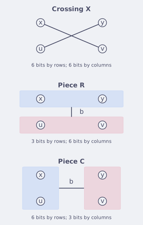
The original crossing needs six bits across either partition. In the signed decomposition $2X=R+C$, $R$ has a three-bit row factorization and $C$ a three-bit column factorization. The shaded groups show those favorable partitions. The pieces may be negative; the picture denotes an algebraic identity, not a disjoint union of satisfying assignments.

Proof of the finite cancellation identity

Write $p=(p_1,p_2,p_3)$ and $q=(q_1,q_2,q_3)$. One explicit choice is $\sigma (p,q)=(-1{)}^{\varphi (p,q)}$, with the following expression computed modulo two:

$$\begin{array}{rl}\varphi (p,q)=& \sum _{1\le i\le j\le 3}{p}_i{q}_j\\ & +q_1{p}_2{p}_3+p_1{q}_2{p}_3\\ & +p_1{p}_2{q}_3.\end{array}$$

Both $R$ and $C$ vanish unless $x\oplus y\oplus u\oplus v=0$. When that parity condition holds and $y=u$, we also have $x=v$, and both signs are $1$.

Otherwise write $d=y\oplus u=x\oplus v\ne 0$. Expanding the four sign exponents modulo two gives

$$\begin{array}{rl}& \varphi (x,y)+\varphi (v,u)\\ & +\varphi (x,u)+\varphi (v,y)\\ & =1+\prod _{j=1}^3(1+d_j)=1.\end{array}$$

The two signs are therefore opposite. Thus $R+C$ is two on the crossing equalities and zero everywhere else. This is a finite identity on $8^4=4096$ inputs; the accompanying script checks every input using exact integer arithmetic.

🏷️ Grouping the expansion without losing the saving

Applying $R+C=2X$ separately to many three-bit blocks would create exponentially many terms. That would impose a positive exponential cost before recursion even begins.

The paper groups terms by the number of blocks using $C$. Pad each $\lambda$-bit string with zeros to $3t$ bits, where $t=\lceil \lambda /3\rceil$. Define $A_i$ by the polynomial identity

$$\begin{array}{c}\prod _{s=1}^t(R_s+T{C}_s)=\sum _{i=0}^t{A}_i{T}^i,\\ \sum _{i=0}^t{A}_i=2^{t}X.\end{array}$$

For a fixed input, all coefficients can be computed by ordinary polynomial multiplication in time polynomial in $\lambda$. There are only $t+1$ pieces.

To factor $A_i$ by rows, specify which $i$ blocks use $C$. Naming that subset costs at most $t$ bits. The remaining indices cost three bits for each $R$ block and six for each $C$ block. Consequently,

$$\begin{array}{rl}{c}_i^{\mathrm{row}}& \le \min \{2\lambda ,4t+3i\},\\ c_i^{\mathrm{col}}& \le \min \{2\lambda ,7t-3i\}.\end{array}$$

Adding the two bounds eliminates $i$:

$$\begin{array}{rl}{c}_i^{\mathrm{row}}+c_i^{\mathrm{col}}& \le 11t\\ & \le \frac{11}{3}\lambda +8.\end{array}$$

The original crossing costs $4\lambda$ across the two partitions together. The new pieces have a combined cost at most a fraction $\rho =11/12$ of that, up to rounding.

The extra bits naming the subset are essential. Ignoring them would overstate the saving. This elementary accounting also explains the choice of eight squares: for two-bit blocks, the four-square identity gives $2+4+1+1=8$ bits against an original cost of eight. Three-bit blocks give $3+6+1+1=11$ against twelve. The paper notes that finer rank calculations can improve other constructions; the comparison here concerns this explicit factorization.

🏷️ A recursion with a vanishing exponential coefficient

The recursive input is a complete graph on $K$ vertices, with $\lambda$ equality bits on each edge and arbitrary integer weights at its vertices. Smaller edges can be padded with bits forced to zero. Its total number of independent edge bits is $\left(\genfrac{}{}{0ex}{}{K}{2}\right)\lambda$.

Call $(K,e)$ achievable when this weighted counting problem can be evaluated using

$$2^{e{K}^2\lambda }\mathrm{poly}(\lambda +B)$$

operations and weight queries, where $B$ bounds the bit length of each supplied weight. The tables are accessed through evaluation procedures, and the cost of those procedures is charged when this intermediate bound is applied. Constants may depend on the fixed pair $(K,e)$. Exhaustive enumeration makes $(K,1/2)$ achievable.

Put $g^2$ vertices on a $g\times g$ grid. Every edge joining different rows and different columns belongs to the diagonal pair of exactly one rectangle. Apply the grouped identity to each rectangle. For a fixed choice of pieces, compare the total row and column costs and merge in the cheaper direction.

The normalization is retained exactly. If $r={\left(\genfrac{}{}{0ex}{}{g}{2}\right)}^2$ is the number of rectangles, the expansion gives $2^{tr}Z={\sum }_{\iota }{Z}_{\iota }$, where $\iota$ chooses a piece for each rectangle. After evaluating and adding the recursive terms, divide by $2^{tr}$. The identity guarantees that this division has an integer result.

The combined-cost inequality ensures that one direction saves a constant fraction of the diagonal bits. Edges already lying in a row or column form a lower-order contribution when $g$ is large.

The resulting edges need not have equal lengths. Padding immediately to the largest length could erase the saving. A second grouping balances the load: merge the $g$ vertices into $K$ groups whose sizes and pairwise boundary costs are controlled. A probabilistic existence argument proves that a good grouping exists; exhaustive search over groupings makes the construction deterministic.

Exponent improvement, Proposition 3

If $(K,e)$ is achievable and $g=3K^8$, then $(g^2,e^{\prime })$ is achievable, where

$$e^{\prime }=\left(\frac{11}{12}+\frac{2}{K}\right)e+\frac{2}{K}.$$

The last term includes the cost of evaluating the weights created by merging. It cannot be dropped.

Starting from $K_0=64$ and $e_0=1/2$, define

$$\begin{array}{rl}{K}_{\ell +1}& =9K_{\ell }^{16},\\ e_{\ell +1}& =\left(\frac{11}{12}+\frac{2}{K_{\ell }}\right)e_{\ell }+\frac{2}{K_{\ell }}.\end{array}$$

Then $K_{\ell }$ grows rapidly and $e_{\ell }\to 0$. Indeed, the multiplicative coefficient is eventually bounded by a constant less than one, while the additive term tends to zero. Iterating this inequality bounds the tail by a decaying geometric term plus an arbitrarily small geometric sum.

At a fixed level, the number of rectangles is fixed. The number of expanded terms,

$$(t+1{)}^{{\left(\genfrac{}{}{0ex}{}{g}{2}\right)}^2},$$

is therefore polynomial in $\lambda$, although its degree is enormous. This order of quantifiers is the reason the expansion does not defeat the qualitative theorem: choose the recursion level for the desired $\delta$, then let the input size grow.

A preliminary balanced grouping converts the clause network into one of these complete-graph instances. The clause count is evaluated in time with exponent $O((e_{\ell }+1/K_{\ell })m)$, apart from factors polynomial in the input for fixed $\ell$. Since both coefficients vanish, the algorithm achieves every positive exponential rate in $m$.

To pass to arbitrary clause density, use count-preserving sparsification. For fixed width and every $\epsilon >0$, it decomposes a formula into at most $2^{\epsilon n}$ sparse formulas with disjoint sets of satisfying assignments. Their counts can therefore be added. The disjointness is important: a decision-only disjunction would not by itself preserve counts. (Impagliazzo, Paturi & Zane, 2001; Dell et al., 2014)

🏷️ The sharper rate and the role of partition numbers

The elementary recursion establishes the failure of ETH, but does not yet yield the main theorem’s square-root logarithmic saving. When the level grows with the input, previously hidden constants and polynomial degrees must be counted explicitly.

Appendices A and B make two additional improvements. Sharper concentration bounds let the next graph size be essentially the square of the previous one, up to polylogarithmic factors. A different family of crossing decompositions improves the contraction factor to

$$\rho =\frac{1}{\sqrt{2}}.$$

These decompositions use operators on the polynomial ring $\mathbb{Q}[t_1,t_2,\dots ]$, graded by $\mathrm{deg}{t}_j=j$. The weight-$h$ component has dimension $p(h)$, the number of integer partitions of $h$. Choose the least $h\ge 2$ such that $p(h)\ge 2^{\lambda }$; the Hardy–Ramanujan estimate $\log p(h)=\Theta (\sqrt{h})$ makes $h=\Theta ({\lambda }^2)$. The construction has $O({\lambda }^2)$ pieces, with factorization dimensions controlled by partition counts.

The new relation between level and graph size gives

$$\begin{array}{rl}\log K_{\ell }& =\Theta (2^{\ell }),\\ e_{\ell }& =\Theta (2^{-\ell /2})\\ & =\Theta ((\log K_{\ell }{)}^{-1/2}).\end{array}$$

Accounting for all construction costs and choosing $K_{\ell }$ as a suitable small power of the input size yields the clause bound $2^{O(km/\sqrt{\log m})}$.

The variable bound needs more than substituting a sparsification estimate for $m$. As $\epsilon$ tends to zero, the maximum occurrence count $\Delta$ produced by sparsification grows too quickly for that substitution. Appendix D constructs a network based on variables, with only $O(kn\log \Delta )$ boundary bits. It combines truncated inclusion–exclusion with sparse parity checks that eliminate assignments violating too many clauses. With the chosen sparsification parameters, $\log \Delta =O(k\log \log n)$ in the relevant range, producing the factor $k^2\log \log n$.

These appendices supply substantial additional arguments. The eight-square calculation explains the mechanism of the ETH refutation; the stronger theorem also needs the partition-based decomposition and the improved treatment of dense formulas. (Claude, 2026)

🏷️ Consequences for counting, search, and graph problems

For every fixed $k$, the theorem gives $s_k=0$. Hence ETH and SETH are false, as is their counting analogue $\#\mathrm{ETH}$. Since the algorithm is deterministic, allowing randomization cannot restore a positive exponential lower bound for these problems.

After establishing satisfiability, search follows by fixing variables one at a time. Ask whether a satisfying assignment exists with the next variable zero; retain zero if it does, and otherwise retain one. At most $n$ further calls recover a witness. This polynomial overhead preserves the stated subexponential rates.

For graph consequences, let $N$ be the number of vertices, $s$ a requested set size, and $q$ a fixed number of colors. Section 7 proves that for every $\delta >0$ the following counts can be computed in $O(2^{\delta N})$ time:

Count	Encoding or reduction
Independent sets of size $s$	One variable per vertex; forbid choosing both ends of an edge
Cliques of size $s$	Independent sets in the complement graph
Vertex covers of size $s$	Complements of independent sets of size $N-s$
Dominating sets of size $s$	Domination clauses, followed by a controlled reduction of wide clauses
Proper $q$-colorings	A fixed number of Boolean indicators per vertex

Here an independent set contains no edge; a vertex cover meets every edge; and a dominating set contains, or has a neighbor of, every vertex. In a proper coloring, adjacent vertices receive different colors. The sets and colorings being counted are labeled.

For independent sets, the clauses are simply

$$\neg x_u\vee \neg x_v(\{u,v\}\in E).$$

There are $N$ selection variables even if the graph is dense. Requiring exactly $s$ selected vertices can be implemented with an $O(N)$-gate bounded-fan-in circuit: a balanced addition tree sums the input bits, followed by comparison with $s$.

Introduce a variable for each gate and clauses enforcing its equivalence to its Boolean function. Every input assignment then has exactly one extension to the gate variables. This gives a count-preserving 3-CNF with $O(N)$ variables, plus the edge clauses. The variable bound handles its possible quadratic clause count.

For fixed $q$, color indicators use $qN=O(N)$ variables. Each vertex must have exactly one color, and each edge forbids equal colors at its endpoints. The resulting width is bounded in terms of $q$, so the theorem applies.

Wide clauses for dominating sets

Domination is expressed by one clause per vertex:

$$x_v\vee \underset{u\in N(v)}{\bigvee }{x}_u.$$

These clauses can have unbounded width. Fix a constant threshold $w$ and choose $w$ literals of a clause that is too long. Partition the assignments into two cases: at least one chosen literal is true, or all $w$ chosen literals are false.

In the first branch replace that clause by the disjunction of its chosen literals. In the second fix those $w$ variables to false and simplify. These cases are disjoint. Along a branch there are at most $N$ first choices, one for each original clause, and at most $N/w$ second choices, since each fixes $w$ previously unassigned variables.

The resulting search tree has at most $2^{O(N\log w/w)}$ leaves. Each leaf has bounded-width clauses and $O(N)$ variables, including the exact-cardinality circuit. Choose $w$ large enough to spend less than half the desired exponent on branching, then apply the fixed-width counting algorithm with the remaining budget. Adding the leaf counts gives $O(2^{\delta N})$. (Claude, 2026, p.C orollary 7)

Testing whether these counts are positive gives decision algorithms. Trying the possible sizes gives optimization algorithms with the same qualitative rate. None of these statements asserts fixed-parameter tractability in the requested clique size: subexponential dependence on the total vertex count and a bound of the form $f(s)N^{O(1)}$ are different requirements.

🏷️ Circuit lower bounds and conditional hardness

There is also a consequence in the opposite direction: a faster algorithm implies that some functions need larger circuits.

Let ${\mathsf{E}}^{\mathsf{NP}}$ be the class of languages decidable in deterministic time $2^{O(N)}$ with an NP oracle. Let $\mathrm{SIZE}(O(N))$ denote languages whose length-$N$ membership functions have Boolean circuits of linear size, with a possibly different circuit at every length.

Williams proved that failure of ETH implies

$${\mathsf{E}}^{\mathsf{NP}}⊈\mathrm{SIZE}(O(N)).$$

His argument assumes small circuits, uses them to encode witnesses for long computations, and checks their validity through a sufficiently fast satisfiability algorithm. The resulting nondeterministic simulation would violate a time hierarchy theorem. The new SAT algorithm supplies the missing hypothesis of that implication. (Williams, 2013)

This conclusion concerns linear-size circuits for a language in ${\mathsf{E}}^{\mathsf{NP}}$. It does not assert superpolynomial circuit lower bounds for NP or resolve $\mathsf{P}$ versus $\mathsf{NP}$.

The effect on earlier conditional lower bounds requires equal care. A theorem of the form

$$\begin{array}{c}\mathrm{ETH}⟹\\ \text{a running-time lower bound}\end{array}$$

remains a valid implication. Once ETH is false, that implication supplies no reason for believing its conclusion. The conclusion itself may still hold for another reason; it must be examined separately.

Likewise, SETH implies the Orthogonal Vectors Hypothesis, which posits the absence of truly subquadratic algorithms for detecting an orthogonal pair between two sets of Boolean vectors in specified growing dimensions. Refuting SETH does not refute this weaker hypothesis. Thus an edit-distance hardness result independently based on Orthogonal Vectors does not disappear merely because its SETH-based justification does. The paper explicitly distinguishes these cases.

🏷️ Integer factorization and the size of a reduction

Let $M$ be a positive integer of bit length

$$L=\lceil {\log }_2(M+1)\rceil .$$

To find a nontrivial factor, encode the relation

$$ab=M,1<a\le b<M.$$

Use Boolean variables for the bits of $a,b$ and a circuit that checks multiplication and the inequalities. A Tseitin encoding introduces gate variables and constant-width clauses enforcing the circuit. With equivalences at every gate, each valid factor pair has a unique extension. Decision and successive bit fixing therefore recover factors.

The essential parameter is the number of variables and clauses after introducing those gates.

Suppose a polynomial-time construction supplies a verification circuit with $S(L)$ bounded-fan-in gates, including the comparisons and with $S(L)\ge L$. Its encoding has $O(S(L))$ variables and clauses. Applying the clause bound gives

$$T_{\mathrm{factor}}(L)\le 2^{O(S(L)/\sqrt{\log S(L)})},$$

with polynomial overhead absorbed into the exponent. Repeatedly finding factors, until all remaining factors are prime, also adds only polynomially many calls. This bound is a consequence obtained by composing reductions; it is not a factoring theorem stated in the paper.

For the elementary schoolbook multiplier, $S(L)=O(L^2)$, so this calculation gives

$$2^{O(L^2/\sqrt{\log L})}.$$

That bound does not improve even on exhaustive trial division, which takes $2^{O(L)}$ time. Faster multiplication circuits can reduce the encoding size, but their gate count must be inserted into the formula; a polynomial reduction alone is insufficient. In general, $2^{o(L^c)}$ need not be subexponential in $L$.

Even a hypothetical linear-size multiplication encoding would only yield the displayed guarantee

$$2^{O(L/\sqrt{\log L})},$$

which is still far from polynomial time. For comparison, the classical general number field sieve already has the heuristic running-time scale

$$\exp \left(O((\ln M{)}^{1/3}(\ln \ln M{)}^{2/3})\right),$$

or $2^{O(L^{1/3}(\log L{)}^{2/3})}$ in terms of bit length. That is a smaller asymptotic exponent than the guarantee from the hypothetical linear-size encoding. Its analysis is heuristic, whereas the SAT theorem is a proved worst-case bound, so these are distinct kinds of guarantees. (Pomerance, 1996)

Consequence for factoring and cryptography

The paper supplies a new general method for solving Boolean constraint problems. It does not supply a practical large-integer factorization algorithm, a polynomial-time classical factoring algorithm, or an RSA attack. Establishing an improvement through SAT requires an efficient encoding and a complete comparison with existing factoring algorithms.

The same accounting applies to other cryptographic searches. If a key has $L$ bits but checking it requires $S$ circuit gates, the SAT theorem is controlled by $S$ after encoding. It does not automatically turn a $2^L$ key search into a subexponential search in $L$.

🏷️ The Lean theorem and the verification boundary

The accompanying formalization separates a readable statement file from the proofs. At the reviewed commit, the principal declarations in Solution.lean are

theorem MainResults.ethIsFalse :
    MainResults.ETHIsFalse := ...
 
theorem MainResults.mainTheorem :
    MainResults.MainTheorem := ...

The ellipses here abbreviate the supplied proof terms; they are not holes in those declarations.

MainTheorem quantifies over one deterministic machine and one absolute constant before quantifying over $k$ and the input formula. It counts steps of Mathlib’s finite-program, multi-stack Turing machine, requires every stack alphabet to be finite, and specifies the binary output encoding of the exact count. Its input conditions include distinct clauses, occurrence of all $n$ variables, and the small-parameter bounds stated earlier.

The successful CI run for commit 16a5ce4 built the development and ran Comparator. Its downloaded configuration permits only propext, Quot.sound, and Classical.choice; its log records acceptance by both Lean’s default kernel and the independent nanoda kernel. The two sorry warnings come from Challenge.lean, which contains the reference statements for comparison. They are not dependencies accepted in the solution proofs.

There are still precise boundaries to the claim. The formal machine model and input encoding are explicit. Their conventional simulation on a word RAM and translation from the paper’s ordinary formula representation are described in the statement file but are outside the formalized propositions. Appendix E also records differences between the paper’s exposition and the Lean development.

For this note, the theorem statements, selected proof mechanisms, and published CI artifacts were checked; the full development was not independently rebuilt. The finite algebra below is an additional local check, not a substitute for the complexity proof. The paper attributes discovery of the core algorithm to an internal Claude model and describes subsequent human collaboration on the presentation.

🏷️ Exact finite verification

The accompanying Python script evaluates the explicit sign formula and verifies $R+C=2X$ on all 4096 three-bit inputs. It also computes the two matrix ranks of each piece using exact rational elimination:

Function	Row rank	Column rank
$X$	64	64
$R$	8	64
$C$	64	8

These ranks agree with the three-bit and six-bit factorizations used above. The script checks a two-block grouped expansion as well, including inputs on which nonzero signed pieces cancel, and generates the figure. All identity and rank checks use exact arithmetic.

The computation verifies the small algebraic component and illustrates the source of the saving. It does not benchmark the full SAT algorithm or establish its asymptotic recurrence experimentally.

Links

• Exact quantum factoring over a fixed finite gate set discusses factoring in a quantum computational model. Its resource guarantees must be distinguished from classical SAT reductions.
• Depth-three circuits beyond the square-root exponent studies size lower bounds for restricted circuits. It provides a comparison with the unrestricted linear-size lower bound for ${\mathsf{E}}^{\mathsf{NP}}$ obtained here through Williams’s implication.

📚 References

🐻  Austrin, P., Kaski, P. & Kubjas, K. 2022. Tensor Network Complexity of Multilinear Maps. Theory of Computing 18(16), 1–54.

🐻  Baez, J.C. 2002. The Octonions. Bulletin of the American Mathematical Society 39(2), 145–205.

🐻  Claude 2026. A 2^o(n) Time Algorithm for 3-SAT.

🐻  Dell, H., Husfeldt, T., Marx, D., Taslaman, N. & Wahlén, M. 2014. Exponential Time Complexity of the Permanent and the Tutte Polynomial. ACM Transactions on Algorithms 10(4), 21:1-21:32.

🐻  Impagliazzo, R. & Paturi, R. 2001. On the Complexity of k-SAT. Journal of Computer and System Sciences 62(2), 367–375.

🐻  Impagliazzo, R., Paturi, R. & Zane, F. 2001. Which Problems Have Strongly Exponential Complexity? Journal of Computer and System Sciences 63(4), 512–530.

🐻  Paturi, R., Pudlák, P., Saks, M.E. & Zane, F. 2005. An Improved Exponential-Time Algorithm for k-SAT. Journal of the ACM 52(3), 337–364.

🐻  Pomerance, C. 1996. A Tale of Two Sieves. Notices of the American Mathematical Society 43(12), 1473–1485.

🐻  Williams, R. 2013. Improving Exhaustive Search Implies Superpolynomial Lower Bounds. SIAM Journal on Computing 42(3), 1218–1244.