3SUM and APSP through sparse lopsided triangles

Overview

Alman and Vassilevska Williams give polynomial savings for two central algorithmic problems: deciding whether three integers sum to zero, and finding all shortest-path distances in a directed graph with integer edge weights. Their paper obtains these improvements from a matrix algorithm that computes a prescribed sparse set of entries without constructing the whole product. The proof combines Schönhage’s ten-product identity, a restriction that removes its error terms exactly, and a count of the recursion leaves shared by many outputs. (Alman & Vassilevska Williams, 2026)

🏷️ Computational problems and polynomial savings

The 3SUM problem asks whether a list of $n$ numbers contains three entries at distinct positions whose sum is zero. A standard equivalent formulation gives three lists and asks for $a+b+c=0$, with one entry from each list. Sorting followed by a two-pointer search gives a quadratic algorithm.

The all-pairs shortest paths problem, APSP, takes a directed graph with edge weights and returns the minimum path weight between every ordered pair of vertices. We assume there are no negative cycles; an unreachable pair has distance $+\infty$. The familiar Floyd–Warshall algorithm uses $O(n^3)$ operations.

The related min-plus product of two matrices is

$$(A\star B{)}_{ij}=\underset{1\le k\le n}{\min }(A_{ik}+B_{kj}).$$

Here addition combines two path segments and minimization selects the best intermediate vertex. This differs from the ordinary arithmetic product

$$(XY{)}_{ij}=\sum _{k=1}^D{X}_{ik}{Y}_{kj},$$

which will be the algebraic engine of the new algorithms.

A running time is truly subquadratic if it is $O(n^{2-\delta })$ for a fixed $\delta >0$, and truly subcubic if it is $O(n^{3-\delta })$. A logarithmic improvement such as $n^2/\log n$ does not have this property. The notation $\tilde{O}$ suppresses polylogarithmic factors; $n^{o(1)}$ permits any subpolynomial factor.

The integer results use a word RAM with $O(\log n)$-bit words. Input numbers have absolute value at most $n^{\nu }$ for a fixed constant $\nu$. Controlling intermediate bit lengths is part of the proof.

Integer consequences

For polynomially bounded integer inputs, the paper gives deterministic algorithms with the following running times:

Problem	Running time
3SUM	$O(n^{1.9992})$
Min-plus product	$O(n^{2.99942})$
Directed APSP, without negative cycles	$O(n^{2.99942})$

The abstract states the slightly weaker APSP bound $O(n^{2.9995})$. The sharper number above is the explicit bound in the theorem on 3SUM and APSP in Section 3.4. (Alman & Vassilevska Williams, 2026)

The 3SUM and APSP hypotheses asserted that no fixed polynomial saving was possible in these integer models. The exponents above refute those hypotheses. Their significance is asymptotic: the theorem does not provide a practical crossover size or an implementation benchmark.

🏷️ Thin products and lopsided triangle queries

Let

$$X\in {\mathbb{Z}}^{N\times D},Y\in {\mathbb{Z}}^{D\times N},$$

where $D$ is a small power of $N$. Such a product is thin because its inner dimension is much smaller than its outer dimensions. Let $W\subseteq [N]\times [N]$ be a specified set of positions. We want only $(XY{)}_{ij}$ for $(i,j)\in W$. Neither input matrix nor the full product is assumed sparse.

The graph interpretation makes the query set natural. Consider an unweighted, undirected tripartite graph with parts $A,M,B$, of sizes $N,D,N$. Let $X$ and $Y$ be the adjacency matrices between $A,M$ and $M,B$. For $a\in A$ and $b\in B$,

$$(XY{)}_{ab}=|\Gamma (a)\cap \Gamma (b)\cap M|.$$

If $W$ is the set of edges between $A$ and $B$, this number counts the triangles containing each edge of $W$. Testing whether the count is positive solves Lopsided All-Edges Sparse Triangle. Equivalently, the neighborhoods are two families of sets over a universe of size $D$, and $W$ specifies offline set-intersection queries.

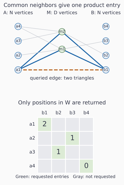
A query edge between the two large parts asks for common neighbors in the small middle part. The algorithm computes exactly these selected entries of the arithmetic product.

Sparse entries of a thin product

Suppose $N\ge D^{18}$, the entries of $X,Y$ have absolute value $N^{O(1)}$, and

$$|W|\le \frac{N^2}{\sqrt{D}}.$$

The wanted entries can be computed deterministically in

$$O\left(\frac{N^2}{D^{0.063}}\right)$$

operations on $O(\log N)$-bit integers. The positions in $W$ may be arbitrary. (Alman & Vassilevska Williams, 2026 s 2 and 4)

At the largest allowed query-set size, computing each entry separately costs $|W|D=N^2\sqrt{D}$. Computing all entries incurs an $N^2$ output cost. The new algorithm beats both because its output has only $N^2/\sqrt{D}$ entries. There is no conflict with an output-size lower bound.

Two qualifications are useful. A polynomial saving in $N$ follows when $D=N^{\epsilon }$ for a fixed $\epsilon >0$; constant $D$ gives only a constant factor. Also, this is sparsity of the requested output positions. An arbitrary dense product is permitted.

We first develop the simpler bound

$$O\left(\frac{N^2{\log }^{2}D}{D^{1/18}}\right),$$

for $D\ge 4$ a power of four. This already gives truly subquadratic 3SUM and truly subcubic APSP. The data structure refinement will explain the exponent $0.063$.

🏷️ Schönhage’s identity and its error structure

Fast matrix multiplication begins with a small bilinear identity and applies it recursively. The additions preparing the scalar multiplications are called encoding; the additions assembling the outputs are decoding. For a sparse-output algorithm, both must be counted.

The starting identity is due to Schönhage, and its recursive use follows the rectangular multiplication approach of Coppersmith. (Schönhage, 1981; Coppersmith, 1982)

Consider two independent tasks:

• the nine entries $x_i{y}_j$ of a $3\times 1$ by $1\times 3$ outer product;
• the inner product ${\sum }_{i,j=1}^2{p}_{ij}{q}_{ij}$ of two four-entry vectors.

Separate evaluation takes thirteen multiplications. Introduce output labels $z_{ij}$ and $z_0$, and encode the desired answers as the coefficients of

$$G=\sum _{i,j=1}^3{x}_i{y}_j{z}_{ij}+\left(\sum _{i,j=1}^2{p}_{ij}{q}_{ij}\right)z_0.$$

Extend the $p$ and $q$ arrays to

$$\begin{array}{c}\hat{p}=\\ \left(\begin{array}{ccc}{p}_{11}& p_{12}& 0\\ p_{21}& p_{22}& 0\\ -p_{11}-p_{21}& -p_{12}-p_{22}& 0\end{array}\right),\end{array}$$ $$\begin{array}{c}\hat{q}=\\ \left(\begin{array}{ccc}{q}_{11}& q_{12}& -q_{11}-q_{12}\\ q_{21}& q_{22}& -q_{21}-q_{22}\\ 0& 0& 0\end{array}\right).\end{array}$$

Every column of $\hat{p}$ and every row of $\hat{q}$ sums to zero. Form ten products, indexed by labels $P_{ij}$ and $P_0$:

$$\begin{array}{rl}{s}_{ij}& =(x_i+{\hat{p}}_{ij})(y_j+{\hat{q}}_{ij}),\\ s_0& =-\left(\sum _{i=1}^3{x}_i\right)\left(\sum _{j=1}^3{y}_j\right).\end{array}$$

The identity is

$$\sum _{i,j=1}^3{s}_{ij}(z_{ij}+z_0)+s_0{z}_0=G+E,$$

where

$$E=\sum _{i,j=1}^3\left(x_i{\hat{q}}_{ij}+{\hat{p}}_{ij}{y}_j+{\hat{p}}_{ij}{\hat{q}}_{ij}\right)z_{ij}.$$

The coefficient of $z_0$ is exactly the desired inner product. Indeed, $s_0$ cancels all $x_i{y}_j$ terms, and the zero row and column sums cancel the cross terms. The remaining sum ${\sum }_{i,j}{\hat{p}}_{ij}{\hat{q}}_{ij}$ equals ${\sum }_{i,j\le 2}{p}_{ij}{q}_{ij}$.

The outer coefficients still contain errors. Recovering the nine outer-product entries and the inner-product sum exactly therefore requires eliminating $E$. Two features of the identity make this possible:

• Every error monomial has an outer output label $z_{ij}$ and at least one inner input variable $p$ or $q$.
• Each outer output $z_{ij}$ uses only the term $P_{ij}$, whereas the inner output $z_0$ uses all ten terms.

The first feature will remove the errors after restriction. The second will control which recursion leaves a wanted output needs.

🏷️ An exact layer of independent matrix products

Apply the ten-term identity through $L$ recursive levels. A left input is indexed by a length-$L$ string over the seven symbols $x_1,x_2,x_3,p_{11},p_{12},p_{21},p_{22}$. Right inputs use the corresponding $y,q$ symbols, and outputs use the ten $z$ symbols.

The inner set of a string is the set of levels using an inner symbol: $p$ on the left, $q$ on the right, or $z_0$ at the output. Fix an integer $m$ and retain only input strings whose inner sets have exactly $m$ elements. Set every other input to zero.

For each $m$-element set $Q\subseteq [L]$, the retained inputs describe an independent matrix product of shape

$$\begin{array}{c}{N}_0\times D\text{by}D\times N_0,\\ N_0=3^{L-m},D=4^m.\end{array}$$

The outer levels specify row and column indices in base three; the inner levels specify the summation index using four choices per level. There are

$$K=\left(\genfrac{}{}{0ex}{}{L}{m}\right)$$

such products.

Exactness of the fixed layer

After zeroing all input strings outside the layer with exactly $m$ inner levels, every output string with inner set $Q$, $|Q|=m$, equals the corresponding entry of $X_Q{Y}_Q$.

To prove this, consider a monomial contributing to such an output. At every level in $Q$, its output symbol is $z_0$. The one-level identity forces both input symbols there to be a matching pair $p_{ij},q_{ij}$. Thus both input strings already have $m$ inner symbols.

Since only inputs with exactly $m$ inner symbols remain, all other levels must use outer inputs. Every error monomial requires an inner input at an outer output level, so none can survive. At an outer level with output $z_{ij}$, the only remaining monomial is $x_i{y}_j{z}_{ij}$. Summing over the four choices at each of the $m$ inner levels gives exactly the desired matrix entry.

This argument also prevents interference between different sets $Q$. Exactness comes from the restriction and the structure of the error monomials; no limiting parameter or floating-point approximation is used.

The recursion therefore provides $K$ independent products at once. Each output entry is the sum of products at certain leaves of the ten-ary recursion tree. A leaf is a string

$$\begin{array}{c}\tau =({\tau }_1,\dots ,{\tau }_L),\\ {\tau }_{\ell }\in \{P_0,P_{11},\dots ,P_{33}\}.\end{array}$$

If an output string has $z_{ij}$ at level $\ell$, its contributing leaves must choose ${\tau }_{\ell }=P_{ij}$. If it has $z_0$, any of the ten choices is allowed. Consequently, one output depends on $10^m$ leaves.

That number exceeds the $D=4^m$ multiplications in a direct inner product. The gain will come from sharing leaves across outputs.

🏷️ Private leaves and the union bound

Fix an output with inner set $Q$. Its private leaf chooses $P_0$ at every level of $Q$ and the required $P_{ij}$ elsewhere. No other output in the fixed layer uses this leaf.

For any contributing leaf, define its order

$$d=m-\#\{\ell :{\tau }_{\ell }=P_0\}.$$

Its order counts the inner levels where the leaf uses a shared term $P_{ij}$ instead of $P_0$. An output uses

$${\alpha }_d=\left(\genfrac{}{}{0ex}{}{m}{d}\right)9^d$$

leaves of order $d$: choose the $d$ levels and one of nine shared terms at each.

Across the whole recursion, the number of leaves of order $d$ is

$${\beta }_d=\left(\genfrac{}{}{0ex}{}{L}{m-d}\right)9^{L-m+d}.$$

Write

$$M=K{N}_0^2=\left(\genfrac{}{}{0ex}{}{L}{m}\right)9^{L-m}$$

for the total number of output entries in the $K$ products. Then ${\beta }_0=M$. A leaf of order $d$ is used by

$$\left(\genfrac{}{}{0ex}{}{L-m+d}{d}\right)$$

outputs: their inner sets must contain its $m-d$ zero positions, and one chooses the other $d$ inner positions among the remaining levels. This gives the exact incidence identity

$$M{\alpha }_d={\beta }_d\left(\genfrac{}{}{0ex}{}{L-m+d}{d}\right).$$

Now let $U$ be an arbitrary set of wanted outputs within this batch, and let $\mathcal{L}(U)$ be the union of their contributing leaves.

Leaf-count bound

$$|\mathcal{L}(U)|\le \sum _{d=0}^m\min \{|U|{\alpha }_d,{\beta }_d\}.$$

For $L=19m$, this implies

$$|\mathcal{L}(U)|\le 2^{-m/9}(2^m|U|+2M).$$

At a fixed order, we may charge every output for all its leaves, giving $|U|{\alpha }_d$, or count all leaves of that order in the entire batch, giving ${\beta }_d$. Either count is valid for every set $U$, regardless of how its entries are arranged.

The choice $L=19m$ makes the second count decay geometrically:

$$\begin{array}{rl}\frac{{\beta }_d}{{\beta }_{d-1}}& =\frac{9(m-d+1)}{L-m+d}\\ & \le \frac{9m}{18m+1}<\frac{1}{2}.\end{array}$$

Thus ${\beta }_d\le 2^{-d}M$. For $d>m/9$, summing this geometric bound costs less than $2\cdot 2^{-m/9}M$. For $d\le m/9$, use the per-output estimate and the binomial theorem:

$$\begin{array}{rl}& \sum _{d\le m/9}\left(\genfrac{}{}{0ex}{}{m}{d}\right)9^d\\ & \le 72^{m/9}\sum _{d=0}^m\left(\genfrac{}{}{0ex}{}{m}{d}\right)8^{-d}\\ & =72^{m/9}(9/8{)}^m\\ & <2^{8m/9}.\end{array}$$

The first inequality uses $9^d=72^d{8}^{-d}$ and $72^d\le 72^{m/9}$ in the indicated range. The last follows from the exact inequality $72(9/8{)}^9<256$. Combining the two ranges proves the claim.

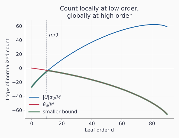
The two leaf-count bounds for $m=90$, $L=19m$, and $|U|=\lfloor M/2^m\rfloor$, divided by $M$ and plotted logarithmically. The lower envelope bounds the required leaves at each order. The proof’s convenient split at $m/9$ need not coincide with the crossing.

Since $2^m=\sqrt{D}$ and $2^{-m/9}=D^{-1/18}$, the estimate becomes

$$|\mathcal{L}(U)|\le D^{-1/18}(\sqrt{D}|U|+2M).$$

For a batch with about $M/\sqrt{D}$ wanted entries, only $O(M/D^{1/18})$ leaves are needed. The estimate is linear in $|U|$, so the same saving survives even if queries are distributed very unevenly among batches.

🏷️ Encoding, pruning, and the full operation count

To apply the construction to $XY$, partition $X$ into row blocks of $N_0$ rows and $Y$ into column blocks of $N_0$ columns. Put

$$K_0=\lfloor \sqrt{K}\rfloor .$$

A tile consists of $K_0$ row blocks and $K_0$ column blocks. Assign its $K_0^2\le K$ block products to distinct $m$-element sets $Q$. Every entry of $XY$ then belongs to one product in one tile.

At a leaf $\tau$, the multiplied numbers have the form ${\Phi }_{\tau }(a)$ and ${\Psi }_{\tau }(b)$, linear functions of the left input array and the right input array separately. All tiles using the same row band have the same left encoding, and similarly for column bands. Computing these arrays once per band costs

$$O\left(\frac{N10^L}{K_0{N}_0}\right),$$

instead of paying for a complete encoding in every tile.

For $L=19m$, the assumption $N\ge D^{18}$ ensures that a tile fits after constant-factor padding and that this encoding cost is $O(N^2{D}^{-1/18})$. One sufficient inequality is

$$10^L\le 2^{-m/9}N{N}_0.$$

It follows by comparing exponential bases:

$$\frac{10^{19}{2}^{1/9}}{3^{18}}<4^{18}.$$

After encoding, the decoder receives only the wanted output strings. At each recursive vertex, let $S_z$ be the wanted suffixes beginning with symbol $z$. The requests sent to its children are

$$\begin{array}{rl}{S}_{P_{ij}}& =S_{z_{ij}}\cup S_{z_0},\\ S_{P_0}& =S_{z_0}.\end{array}$$

An empty request set requires no recursive call. The unions are essential: a child used by several outputs is evaluated once.

There is a second counting argument for the decoder’s additions and bookkeeping. At a fixed depth, map each requested suffix to its private completion: retain the existing leaf prefix, then replace $z_0$ by $P_0$ and $z_{ij}$ by $P_{ij}$ in the suffix. The completion is a leaf in $\mathcal{L}(U)$ and determines both the vertex and suffix. Hence the total size of request sets at each depth is at most $|\mathcal{L}(U)|$.

There are $L+1$ depths, and sorted-list operations on length-$L$ strings take $O(L)$ time per handled string. The full pruned computation therefore costs

$$O(L^2|\mathcal{L}(U)|)$$

per tile. Summing the leaf bound over tiles, using ${\sum }_T|U_T|=|W|$ and ${\sum }_{T}M=O(N^2)$, gives

$$O\left(\frac{N^2{\log }^{2}D}{D^{1/18}}\right).$$

The remaining input and indexing costs fit within this bound. Encoded values are signed sums of at most $7^L$ input entries; decoded values are sums of at most $10^L$ products of two encoded values. These counts are polynomial in $N$, so polynomially bounded inputs produce only $O(\log N)$-bit intermediate integers.

🏷️ Online queries and the improved exponent

The preceding decoder knows $W$ in advance. The stronger result preprocesses $X,Y$ before any query positions are supplied.

For an output with inner set $Q$, its $10^m$ contributing leaves form a discrete cube: the choices at levels in $Q$ are free, while all other levels are fixed. Choose an integer switching order $1\le t\le m$. Evaluate leaves of order below $t$ individually at query time, and group the higher-order leaves into precomputed partial sums called boxes.

A box is a string over the ten term labels and a wildcard $\ast$. A wildcard permits all ten labels, including $P_0$. Require that at most $m-t$ symbols are either $P_0$ or wildcards, and that every wildcard occurs at a lower-numbered level than every $P_0$.

To assign a contributing leaf of order at least $t$ to a box, scan its inner levels from highest to lowest until the $t$-th nonzero label $P_{ij}$ is reached. Keep everything scanned, and replace all remaining lower inner levels by wildcards. This assigns each such leaf to exactly one box for the given output. The number of boxes needed by one output is

$${\alpha }_t=\left(\genfrac{}{}{0ex}{}{m}{t}\right)9^t.$$

For example, with four inner levels and $t=2$, the string

$$(P_{12},P_0,P_{31},P_{22})$$

belongs to the box

$$(\ast ,\ast ,P_{31},P_{22}).$$

Its first two positions range over all $10^2$ possibilities. Boxes are identified by their strings, so the same stored sum can serve several outputs.

Across a tile, there are at most

$$(m+1)\sum _{d=t}^m{\beta }_d$$

boxes. To see the count, replace all wildcards of a box by $P_0$. This gives a leaf of order at least $t$. The original box is recovered by turning some initial segment of that leaf’s $P_0$ positions into wildcards, with at most $m+1$ choices.

The box values are computed by dynamic programming. Replace the highest wildcard by each of the ten term labels and sum the resulting values. Each child is again a valid box with one fewer wildcard. This preserves the ordering condition and gives constant branching.

For general $L$, put

$$\rho =\frac{9m}{L-m+1}.$$

When $L>10m$, we have $\rho <1$ and ${\beta }_d\le {\rho }^{d}M$. Assume also $N\ge \sqrt{K}{N}_0$, so that a tile fits after constant-factor padding. The preprocessing and query bounds are

$$\begin{array}{rl}P(N,D)& =O\left(\frac{Lm{\rho }^t}{1-\rho }{N}^2\right)\\ & +O\left(\frac{N10^L}{\sqrt{K}{N}_0}\right),\\ Q(D)& =O\left(L\sum _{d=0}^t\left(\genfrac{}{}{0ex}{}{m}{d}\right)9^d\right).\end{array}$$

Choose $L=21m$ and $t=\lceil m/9\rceil$. Then $\rho <9/20$, and the two relevant exponents are

$$\begin{array}{rl}{\gamma }_0& =\frac{\log (20/9)}{9\log 4}\\ & \approx 0.064000,\\ q_0& =\frac{\log 72+9\log (9/8)}{9\log 4}\\ & \approx \mathrm{0.427736.}\end{array}$$

The encoding term also fits when $N\ge D^{18}$. Absorbing logarithmic factors into the strict margins ${\gamma }_0>0.063$ and $q_0<0.437$ gives

$$\begin{array}{rl}P(N,D)& =O(N^2/D^{0.063}),\\ Q(D)& =O(D^{0.437}).\end{array}$$

Consequently, $|W|\le N^2/\sqrt{D}$ queries take

$$|W|D^{0.437}\le N^2{D}^{-0.063},$$

matching the preprocessing cost. Padding an arbitrary $D$ to the next power of four changes the asymptotic constants; the proof handles bounded $D$ separately.

General range

Let

$${\epsilon }_{\ast }=\frac{\log 4}{5\log 10}\approx \mathrm{0.120412.}$$

For every fixed $0<\epsilon <{\epsilon }_{\ast }$ and $\kappa >0$, some $\gamma >0$ allows all $|W|\le N^2/D^{\kappa }$ wanted entries to be computed in $O(N^2/D^{\gamma })$ time whenever $2\le D\le N^{\epsilon }$. The exponent $\gamma$ depends on the chosen parameters. (Alman & Vassilevska Williams, 2026, sec.4)

The endpoint reflects the encoding cost. As $L/m$ approaches $10$ from above, $M=\left(\genfrac{}{}{0ex}{}{L}{m}\right)9^{L-m}$ approaches $10^L$ up to polynomial factors. Shared encoding then has scale $N10^{L/2}$, which can stay below $N^2$ only when $N$ exceeds approximately $10^{5m}$. Since $D=4^m$, this gives the threshold $\log 4/(5\log 10)$. The strict inequality in the theorem leaves room for a positive saving.

🏷️ Exact Triangle and deterministic modular filtering

Exact Triangle takes a complete tripartite graph with $n$ vertices per part and integer edge weights. It asks whether some triple satisfies

$$\begin{array}{rl}S(a,b,c)& =w(a,b)+w(b,c)\\ & +w(a,c)=0.\end{array}$$

Weights have absolute value at most $n^{\nu }$, for fixed $\nu$. The paper adapts earlier triangle reductions, particularly the deterministic construction of Chan and Xu, to produce lopsided instances. (Chan & Xu, 2024)

Let $16\le D\le n$ and $1\le g\le \sqrt{D}$. Choose a prime $p$ between $\sqrt{D}/2$ and $\sqrt{D}$. Every zero-weight triangle survives reduction modulo $p$; some nonzero-weight triangles may also survive.

Write $F(p)$ for this false-positive count and $Z_0$ for the number of exact zero triangles. The quantity $F(p)+Z_0$ is computable by matrix multiplication over

$$\mathbb{Z}[x]/(x^p-1).$$

For example, the coefficient of $x^r$ in the product of matrices with entries $x^{w(a,c)\mathrm{mod}p}$ and $x^{w(b,c)\mathrm{mod}p}$ counts intermediate vertices whose two weights sum to $r$ modulo $p$. Summing the coefficients indexed by $-w(a,b)$ counts modular zero triangles.

Compute this count for every prime in the indicated interval and select the smallest. Since $Z_0$ is independent of the prime, this also minimizes $F(p)$. Each nonzero integer $S(a,b,c)$ has only

$$O\left(\frac{\nu \log n}{\log D}\right)$$

prime divisors in this interval. Averaging over its $\Omega (\sqrt{D}/\log D)$ primes gives

$$F(p)=O\left(\frac{\nu n^3\log n}{\sqrt{D}}\right).$$

Next, split the third vertex part into pieces $C_k$ of size $O(\sqrt{D}/g)$. Group outer pairs $(a,b)$ by the residue $\varrho =w(a,b)\mathrm{mod}p$, and split each group into chunks of at most $n^2/\sqrt{D}$ pairs.

For each piece and chunk, use the middle vertices $(c,\sigma )\in C_k\times {\mathbb{Z}}_p$, with edges defined by

$$\begin{array}{c}a\sim (c,\sigma )\\ ⟺\sigma \equiv w(a,c)+\varrho (\mathrm{mod}p),\\ (c,\sigma )\sim b\\ ⟺\sigma \equiv -w(b,c)(\mathrm{mod}p).\end{array}$$

A queried pair has a common middle neighbor exactly when some $c$ in the piece completes a modular zero triangle. The middle part has at most $D$ vertices, and the construction produces $O(ng)$ lopsided instances.

For each accepted pair, scan its piece for an exact zero triangle. We stop as soon as an exact zero triangle is found, so there is at most one successful scan. A failed scan contains a false positive, and different failed scans can be charged to different false-positive triples. The total scanning cost is therefore

$$\begin{array}{rl}& O\left((F(p)+1)\frac{\sqrt{D}}{g}\right)\\ & =O\left(\frac{\nu n^3\log n}{g}\right).\end{array}$$

Reduction cost

Exact Triangle reduces deterministically to at most $4ng$ lopsided instances, each with at most $n^2/\sqrt{D}$ queries, plus

$$\begin{array}{c}O\left(\frac{\nu n^3\log n}{g}\right)\\ +O\left(n^{\omega +o(1)}{D}^{3/2}+n^{2}Dg\right)\end{array}$$

additional time. The three terms pay for witness scans, selecting the prime, and constructing the instances. Here $\omega$ is the arithmetic matrix-multiplication exponent. (Alman & Vassilevska Williams, 2026, sec.3.2)

The prime is chosen deterministically, and every candidate is checked against the original weights. Modular collisions affect the running time, not the correctness of the answer.

🏷️ Propagating the exponent savings

Suppose a lopsided instance costs $O(n^2{D}^{-\gamma })$. The oracle calls cost $O(n^{3}g{D}^{-\gamma })$, while witness scans cost $\tilde{O}(n^3/g)$. Taking

$$g\asymp D^{\gamma /2}$$

balances them, leaving a saving $D^{\gamma /2}$.

For $\gamma =0.063$ and $D\asymp n^{1/18}$, this becomes

$${\epsilon }^{\prime }=\frac{0.063}{2\cdot 18}=\mathrm{0.00175.}$$

The prime-selection term is smaller: even Strassen’s exponent ${\log }_{2}7$ gives ${\log }_{2}7+1/12<2.9$. Constructing the instances is also lower order. Thus Exact Triangle takes

$$O(n^{3-0.00175}\log n)\subseteq O(n^{2.9983}).$$

Using the simpler $\gamma =1/18$ algorithm instead gives $O(n^{3-1/648}{\log }^{2}n)$.

The 3SUM reduction

Known deterministic reductions convert a 3SUM input of size $n$ into $n^{1/2+o(1)}$ Exact Triangle instances, each with $n^{1/2+o(1)}$ vertices per part, with $n^{3/2+o(1)}$ additional work. They combine the 3SUM-to-Convolution-3SUM reduction with the weighted-triangle construction. (Chan & He, 2020; Vassilevska Williams & Williams, 2013)

Substituting a triangle exponent $3-{\epsilon }^{\prime }$ gives

$$\begin{array}{rl}& n^{1/2+o(1)}{\left(n^{1/2+o(1)}\right)}^{3-{\epsilon }^{\prime }}\\ & =n^{2-{\epsilon }^{\prime }/2+o(1)}.\end{array}$$

For ${\epsilon }^{\prime }=0.00175$, the exponent is $1.999125+o(1)$, hence the stated $O(n^{1.9992})$ bound. The small slack absorbs the subpolynomial factors.

The min-plus and APSP reductions

If Exact Triangle on $s$ vertices per part takes time $T(s)$, the known reductions give min-plus multiplication in

$$O\left(n^{2}T(n^{1/3}){\log }^{2}U\right),$$

where matrix entries have magnitude at most $U$, and APSP with polynomially bounded integer weights in

$$O\left(n^{2}T(n^{1/3}){\log }^{3}n\right).$$

The applicable reduction assumes $T(s)/s$ is nondecreasing, as it is for the bound used here. (Vassilevska Williams & Williams, 2018; Vassilevska Williams & Williams, 2013)

With $T(s)=O(s^{3-{\epsilon }^{\prime }}\log s)$, both bounds become

$$\tilde{O}(n^{3-{\epsilon }^{\prime }/3}).$$

Since $3-0.00175/3=2.9994166\dots$, this is $O(n^{2.99942})$. The exponent accounting is now explicit: balancing the modular reduction retains half the thin-product saving, the restriction $D\asymp n^{1/18}$ rescales it, and the final reductions retain another half for 3SUM or another third for APSP.

🏷️ Further consequences and the direction of reductions

For real inputs, the paper uses different reductions based on comparison counts and Fredman’s identity

$$\begin{array}{c}{a}^{\prime }+b^{\prime }<a+b\\ ⟺a^{\prime }-a<b-b^{\prime }.\end{array}$$

The resulting algorithms are Las Vegas: they always return the correct answer, with randomized running time. They solve real 3SUM in expected $O(n^{1.998})$ time, and real Exact Triangle, min-plus product, and APSP without negative cycles in expected $O(n^{2.998})$ time. Their only operations on real numbers are comparisons, additions, and subtractions. These bounds arise through the real-input reduction framework, rather than by applying integer modular hashing directly to reals. (Chan, Vassilevska Williams & Xu, 2022; Alman & Vassilevska Williams, 2026, sec.5.2)

There are also deterministic improvements for weighted clique problems. For a fixed $k\ge 3$, partition the chosen vertices into three groups of size $\lfloor k/3\rfloor$, enumerating the remaining one or two vertices if necessary. Group choices become vertices of a triangle instance. Assign its edge weights so that every original edge is counted exactly once. The resulting bound for Zero-Weight $k$-Clique is

$$O\left(n^{k-0.0017\lfloor k/3\rfloor }\right).$$

The paper obtains the same bound for minimum- and maximum-weight $k$-cliques with polynomially bounded integer weights.

The online data structure also refutes rectangular hinted matrix-vector conjectures in sufficiently thin parameter regimes. Here the candidate vectors are supplied as a matrix before a later query identifies the desired vector or entry. That timing allows preprocessing of both factors. It does not give the same result for ordinary online matrix-vector multiplication, where each new vector is unavailable beforehand.

Finally, reduction direction matters. If $A$ reduces to $B$, an algorithm for $B$ yields an algorithm for $A$. An algorithm for $A$ need not yield one for $B$. Consequently, equivalences and reductions to 3SUM, APSP, or the new matrix problem transmit speedups. A one-way proof that a geometric or dynamic problem is 3SUM-hard can lose its conditional lower-bound premise without producing a faster algorithm for that problem.

The paper’s construction also does not handle the balanced sparse-triangle problem at the same improved scale, and does not itself give algorithms refuting the Orthogonal Vectors or SETH hypotheses. The specific thin matrix shape and sparse query set are essential to the argument.

🏷️ Exact finite checks and formalization

The accompanying verification and figure script checks the ten-term identity coefficient by coefficient over the integers, compares small fixed-layer recursive products with direct multiplication, and exhaustively checks the box partition on small cubes. For $m=4,t=2$, the high-order part has

$${\alpha }_2+{\alpha }_3+{\alpha }_4=9963$$

leaves, partitioned into ${\alpha }_2=486$ boxes. These checks verify finite algebra and combinatorics; the asymptotic running-time theorem depends on the general estimates above.

The paper credits an internal Claude model with discovering the initial algorithm, followed by the authors’ work on its analysis, simplification, extensions, and presentation. Its methodology section reports Lean formalizations of the integer Exact Triangle theorem, the integer 3SUM and APSP theorem, and the zero-weight case of the clique corollary, together with their dependencies. It links the 3SUM–APSP formalization. That reported coverage should be distinguished from the additional real-input and online-query results; no independent Lean build is claimed here. (Alman & Vassilevska Williams, 2026)

Links

• Matrix multiplication exponents develops square and rectangular arithmetic exponents. The present algorithm adds a separate resource: the pattern of dependencies between intermediate products and requested outputs.
• on subexponential SAT and its consequences discusses a different algorithmic result concerning satisfiability. The comparison clarifies why improvements for 3SUM and APSP do not, through the reductions in this paper, establish corresponding SAT improvements.

📚 References

🐻  Alman, J. & Vassilevska Williams, V. 2026. Truly Subquadratic 3SUM and Truly Subcubic APSP via Triangles in Sparse Lopsided Graphs.

🐻  Chan, T.M. & He, Q. 2020. Reducing 3SUM to Convolution-3SUM. In 2020 Symposium on Simplicity in Algorithms (SOSA), pp. 1–7.

🐻  Chan, T.M. & Xu, Y. 2024. Simpler Reductions from Exact Triangle. In 2024 Symposium on Simplicity in Algorithms (SOSA), pp. 28–38.

🐻  Chan, T.M., Vassilevska Williams, V. & Xu, Y. 2022. Hardness for Triangle Problems under Even More Believable Hypotheses: Reductions from Real APSP, Real 3SUM, and OV. In Proceedings of the 54th Annual ACM SIGACT Symposium on Theory of Computing, pp. 1501–1514. , Association for Computing Machinery.

🐻  Coppersmith, D. 1982. Rapid Multiplication of Rectangular Matrices. SIAM Journal on Computing 11(3), 467–471.

🐻  Schönhage, A. 1981. Partial and Total Matrix Multiplication. SIAM Journal on Computing 10(3), 434–455.

🐻  Vassilevska Williams, V. & Williams, R. 2013. Finding, Minimizing, and Counting Weighted Subgraphs. SIAM Journal on Computing 42(3), 831–854.

🐻  Vassilevska Williams, V. & Williams, R.R. 2018. Subcubic Equivalences Between Path, Matrix, and Triangle Problems. Journal of the ACM 65(5), 27:1-27:38.