on a metric of positive sectional curvature on S2 x S2

Overview

Brendle and Hung (Brendle & Hung, 2026) construct a metric on $S^2\times S^2$ with positive sectional curvature, resolving in the affirmative the question that has come to be called Hopf’s problem: whether a product of two round spheres admits any metric whose sectional curvature is everywhere strictly positive. The starting point is a Cheeger deformation of the standard product metric — the Cheeger–Müter metric $g$, whose curvature is nonnegative and vanishes exactly on one distinguished two-plane at each generic point (Cheeger, 1973; Müter, 1987; Ziller, 2009). The new metric is a third-order perturbation

$${\tilde{g}}_s=g+s{h}^{(1)}+s^2{h}^{(2)}+s^3{h}^{(3)},$$

whose tensors $h^{(k)}$ are explicit and globally smooth. The argument proceeds in three variations. The first variation of the minimum sectional curvature at each point vanishes; the second variation is nonnegative everywhere and strictly positive away from a single embedded torus $\Sigma$ (the product of two equators); along $\Sigma$ the second variation vanishes, and the perturbation is arranged so that the third variation there is a nonzero constant $\mu$. Consequently the minimum sectional curvature of ${\tilde{g}}_s$ is positive for $s>0$ if $\mu >0$ and for $s<0$ if $\mu <0$, and the main theorem follows.

Two structural ingredients make the mechanism rigorous. The first is an abstract framework for the Taylor expansion of infimum functions $U(x,s)={\inf }_{w}u(x,w,s)$ around a nondegenerate minimum of $u(\cdot ,\cdot ,0)$: it converts pointwise computations of first, second, and third variations of curvature into a clean positivity criterion, and it is what allows the argument to reach the diagonal ${\Delta }_{+}$ and the anti-diagonal ${\Delta }_{-}$, where the coordinate system degenerates, by continuity and density. The second is the linear algebra of metric perturbations — the operators $L$, $Q$, $C$ controlling $R^{(1)},R^{(2)},R^{(3)}$ — which reduces every variation to a finite, explicit computation.

The roadmap of these notes follows the paper: (1) the Cheeger–Müter background metric and its zero-curvature set; (2) the abstract infimum framework; (3) the calculus of metric perturbations and the projection operators; (4) the explicit ansatz $h^{(1)},h^{(2)}$ and the first two variations, including the critical torus $\Sigma$; (5) the third variation and the conformal correction $h^{(3)}=6\chi g$ that makes it constant; (6) the endgame, in which the manifold version of the framework upgrades the pointwise variations to positivity of all sectional curvatures. The authors state that several of the computations (the ten identities for the second variation and the integral ${\pi }^2/(18\sqrt{3})$) were carried out in Mathematica, and the notebook accompanies the preprint.

Preprint status and the stakes

This is arXiv v1 (August 19, 2026) and has not been independently verified. The result, if correct, refutes the long-standing Hopf conjecture that $S^2\times S^2$ admits no metric of positive sectional curvature, and the correctness of the construction rests on a large symbolic computation that the manuscript itself delegates to a Mathematica notebook. The structural parts of the argument — the abstract framework, the curvature linearization, the Cheeger deformation formulas, and every quantity appearing in the first-variation step — are verified independently in the numerical section below; the ten second-variation identities and the integral identity are quoted from the notebook, exactly as the paper does. The reader should treat the positivity claim as provisional pending verification of those identities.

🏷️ The Hopf Problem: Context and Obstructions

A Riemannian manifold $(M,g)$ has positive sectional curvature if every two-plane $\pi \subset T_{p}M$ has sectional curvature

$$K_g(\pi )=\frac{R_g(X,Y,X,Y)}{|X{|}_g^2|Y{|}_g^2-⟨X,Y{⟩}_g^2}>0,$$

where $\{X,Y\}$ is any basis of $\pi$ and $R_g$ is the Riemann curvature tensor, normalized so that the unit sphere has $K\equiv 1$. Compact manifolds admitting such metrics are remarkably rigid: Synge’s theorem forces orientability in odd dimensions (and simple connectivity for orientable even-dimensional ones), the Gauss–Bonnet–Chern theorem forces positive Euler characteristic in even dimensions, and the Bonnet–Myers theorem forces finite fundamental group. In dimension three Hamilton’s classification of positive Ricci curvature shows that a positively curved three-manifold is a quotient of $S^3$ (Hamilton, 1982). In dimension four, Hsiang and Kleiner proved that a positively curved four-manifold admitting a nontrivial Killing field is homeomorphic to $S^4$ or ${\mathbb{CP}}^2$ (Hsiang & Kleiner, 1989) — so any metric of positive curvature on $S^2\times S^2$ must be completely asymmetric, with no continuous isometries. This explains why the construction below systematically breaks the $SO(3)$-symmetry of the background metric, using fixed unit vectors $e_x,e_y,e_z$.

The question itself goes back to Hopf’s work on the interplay between curvature and topology: $S^2\times S^2$ plainly carries metrics of nonnegative sectional curvature — the standard product metric — and Hopf asked whether some metric makes the curvature strictly positive. The early literature approached the problem through perturbations of product metrics (Bourguignon, Deschamps & Sentenac, 1972; Bourguignon, 1975). Cheeger’s construction of nonnegatively curved metrics from group actions produced nontrivial examples on $S^2\times S^2$ (Cheeger, 1973), studied further by Müter (Müter, 1987); Ziller’s notes give a modern account (Ziller, 2009). These Cheeger–Müter metrics are the optimal background for the problem: nonnegatively curved, with a zero-curvature set that is as small as possible — a single plane at each generic point. The methodological ancestor of the present work is the construction of an exotic sphere with positive sectional curvature by Petersen and Wilhelm (Petersen & Wilhelm, 2008), which likewise proceeds by a controlled perturbation of a nonnegatively curved metric (the Gromoll–Meyer sphere (Gromoll & Meyer, 1974)) whose zero-curvature set is well understood.

Main theorem (Brendle–Hung)

There exists a metric on $S^2\times S^2$ with positive sectional curvature.

The main theorem is a direct consequence of the quantitative positivity statement proved at the end: for a suitable choice of the parameters ${\lambda }_c,{\lambda }_d$ there is a constant $\mu \ne 0$ such that ${\tilde{g}}_s$ has positive sectional curvature for all sufficiently small $s>0$ if $\mu >0$ and for all sufficiently small $-s>0$ if $\mu <0$.

🏷️ Preliminaries: The Cheeger–Müter Metric

Throughout, $M=S^2\times S^2$ and $g_{\mathrm{std}}$ denotes the product of unit round metrics, so each factor has Gauss curvature one. The diagonal $SO(3)$ action on $M$ has infinitesimal generators

$$K_{\omega }=(\omega \wedge p_1,\omega \wedge p_2),\omega \in {\mathbb{R}}^3,$$

at $p=(p_1,p_2)$, and we also write

$$J_{\omega }=(\omega \wedge p_1,-\omega \wedge p_2).$$

The diagonal ${\Delta }_{+}=\{p_1=p_2\}$ and the anti-diagonal ${\Delta }_{-}=\{p_1=-p_2\}$ are the two $SO(3)$-orbits of codimension two, and

$$M_{\mathrm{generic}}=M\setminus ({\Delta }_{+}\cup {\Delta }_{-})=\{p_1\ne \pm p_2\}$$

is the open dense subset where the orbit dimension is maximal.

The frame of $M_{\mathrm{generic}}$

On $M_{\mathrm{generic}}$ one fixes a moving frame. Identify $SO(3)$ with ordered orthonormal bases $\mathbf{q}=(q_1,q_2,q_3)$ of ${\mathbb{R}}^3$ satisfying $q_1\wedge q_2=q_3$, and set

$$\begin{array}{rlrl}{q}_1& =\frac{p_1+p_2}{|p_1+p_2|},& q_2& =\frac{p_2-p_1}{|p_2-p_1|},\\ q_3& =\frac{p_1\wedge p_2}{|p_1\wedge p_2|},& \theta & =\frac{1}{2}\arccos ⟨p_1,p_2⟩.\end{array}$$

The map $p\mapsto (\mathbf{q},\theta )$ identifies $M_{\mathrm{generic}}$ with $SO(3)\times (0,\frac{\pi }{2})$, and inverting it gives

$$\begin{array}{rlrl}{p}_1& =\cos \theta q_1-\sin \theta q_2,& p_2& =\cos \theta q_1+\sin \theta q_2,\end{array}$$

so that

$$⟨p_1,p_2⟩=\cos 2\theta .$$

Let $E_1,E_2,E_3$ be the left-invariant vector fields on $SO(3)$ characterized by $E_i{q}_j={\sum }_k{\epsilon }_{ijk}{q}_k$, with dual one-forms ${\sigma }^1,{\sigma }^2,{\sigma }^3$, viewed as fields and forms on $M_{\mathrm{generic}}$. The first identity to record is

$$E_i=(q_i\wedge p_1,q_i\wedge p_2)=K_{q_i},$$

together with ${\partial }_{\theta }=-J_{q_3}$. In these coordinates the standard metric reads

$$\begin{array}{rl}{g}_{\mathrm{std}}=& 2{\sin }^2\theta {\sigma }^1\otimes {\sigma }^1+2{\cos }^2\theta {\sigma }^2\otimes {\sigma }^2\\ & +2{\sigma }^3\otimes {\sigma }^3+2d\theta \otimes d\theta ,\end{array}$$

which one verifies directly from the components of $E_1,E_2,E_3,{\partial }_{\theta }$ in the $q$-frame.

Cheeger deformations

A Cheeger deformation of $g_{\mathrm{std}}$ with parameter $t>0$ is obtained as follows (Cheeger, 1973; Ziller, 2009). Equip $M\times SO(3)$ with the metric $g_{\mathrm{std}}+\frac{1}{t}Q$, where $Q$ is the bi-invariant metric on $SO(3)$ inducing the standard inner product on $\mathfrak{so}(3)\cong {\mathbb{R}}^3$, and let $g_{\mathrm{std},t}$ be the metric on $M$ for which the map $(p,\mathbf{q})\mapsto {\mathbf{q}}^{-1}p$ is a Riemannian submersion. Write ${\mathcal{V}}_p=\mathrm{span}\{K_{\omega }:\omega \in {\mathbb{R}}^3\}$ for the vertical subspace and ${\mathcal{H}}_p$ for its $g_{\mathrm{std}}$-orthogonal complement, and let $P_p$ be the endomorphism of ${\mathcal{V}}_p$ determined by

$$⟨P_p({\omega }_1),{\omega }_2⟩=g_{\mathrm{std}}(K_{{\omega }_1},K_{{\omega }_2})\text{at }p.$$

Ziller’s formula for the deformation is $g_{\mathrm{std},t}(X,Y)=g_{\mathrm{std}}(C_{t}X,Y)$, where

$$C_{t}X=(I+t{P}_p{)}^{-1}{X}^{\mathcal{V}}+X^{\mathcal{H}}$$

for the vertical–horizontal decomposition $X=X^{\mathcal{V}}+X^{\mathcal{H}}$. Since $E_i=K_{q_i}$, the vectors $E_1,E_2,E_3$ are eigenvectors of $P_p$ with eigenvalues $2{\sin }^2\theta$, $2{\cos }^2\theta$, $2$ respectively, and the horizontal direction ${\partial }_{\theta }$ is left untouched by $C_t$. This gives the closed form

$$\begin{array}{rl}{g}_{\mathrm{std},t}=& \frac{2{\sin }^2\theta }{1+2t{\sin }^2\theta }{\sigma }^1\otimes {\sigma }^1+\frac{2{\cos }^2\theta }{1+2t{\cos }^2\theta }{\sigma }^2\otimes {\sigma }^2\\ & +\frac{2}{1+2t}{\sigma }^3\otimes {\sigma }^3+2d\theta \otimes d\theta .\end{array}$$

Two remarks on conventions

The coefficient of $d\theta \otimes d\theta$ deserves comment: the manuscript displays it as $1$, but Ziller’s formula forces it to be $2$ — the direction ${\partial }_{\theta }$ is $g_{\mathrm{std}}$-orthogonal to every orbit direction $K_{\omega }$, as

$$g_{\mathrm{std}}(K_{\omega },{\partial }_{\theta })=-⟨\omega ,q_3⟩+⟨\omega ,q_3⟩=0,$$

hence horizontal, hence fixed by $C_t$, hence $g_{\mathrm{std},t}({\partial }_{\theta },{\partial }_{\theta })=g_{\mathrm{std}}({\partial }_{\theta },{\partial }_{\theta })=2$. The display above uses the corrected coefficient; the manuscript’s normalization $g=\frac{1}{2}{g}_{\mathrm{std},1}$ then gives coefficient $1$ on $d\theta \otimes d\theta$ in $g$, which is the normalization used in every later identity — $|m_4{|}_g^2=1$, ${\rm Y}(y,0)=\frac{1}{3}$, the Laplacian ${\Delta }_{\Sigma }=3m_3^2+m_4^2$, and the conformal identity below. This is verified numerically in the verification section. Also note the bracket convention for the left-invariant frame: $E_i{q}_j={\epsilon }_{ijk}{q}_k$ gives $[E_i,E_j]=+{\epsilon }_{ijk}{E}_k$, which is the convention used in all frame computations below.

Throughout the rest of the construction $g=\frac{1}{2}{g}_{\mathrm{std},1}$ is the background Cheeger–Müter metric,

$$\begin{array}{rl}g=& \frac{{\sin }^2\theta }{2-\cos 2\theta }{\sigma }^1\otimes {\sigma }^1+\frac{{\cos }^2\theta }{2+\cos 2\theta }{\sigma }^2\otimes {\sigma }^2\\ & +\frac{1}{3}{\sigma }^3\otimes {\sigma }^3+d\theta \otimes d\theta .\end{array}$$

It is convenient to rescale the frame to

$$m_1=\frac{1}{\sin \theta }{E}_1,m_2=\frac{1}{\cos \theta }{E}_2,m_3=E_3,m_4={\partial }_{\theta },$$

which is $g$-orthogonal with

$$\begin{array}{rlrl}g(m_1,m_1)& =\frac{1}{2-\cos 2\theta },& g(m_2,m_2)& =\frac{1}{2+\cos 2\theta },\\ g(m_3,m_3)& =\frac{1}{3},& g(m_4,m_4)& =1.\end{array}$$

The orbital fields expand in this frame as

$$K_{\omega }=⟨\omega ,q_1⟩\sin \theta m_1+⟨\omega ,q_2⟩\cos \theta m_2+⟨\omega ,q_3⟩m_3,$$ $$J_{\omega }=⟨\omega ,q_2⟩\cos \theta m_1+⟨\omega ,q_1⟩\sin \theta m_2-⟨\omega ,q_3⟩m_4,$$

identities obtained by expanding $\omega$ in the $q$-basis and using $\omega \wedge p_1=\cos \theta \omega \wedge q_1-\sin \theta \omega \wedge q_2$ together with the exterior products of the $q_i$‘s. For later use, the flat one-forms satisfy

$$\begin{array}{rlrl}{K}_{\omega }^{♭}(m_3)& =\frac{1}{3}⟨\omega ,q_3⟩,& K_{\omega }^{♭}(m_4)& =0,\\ J_{\omega }^{♭}(m_3)& =0,& J_{\omega }^{♭}(m_4)& =-⟨\omega ,q_3⟩.\end{array}$$

The zero-curvature set

Cheeger’s submersion construction — more precisely, Ziller’s quantitative lower bound quoted in the appendix below — gives $K_g\ge 0$ everywhere. The zero-curvature set has a clean description. Let $\mathcal{N}$ denote the Grassmannian of all tangent two-planes of $M$, a compact manifold of dimension $8$; for each $p=(p_1,p_2)$ let

$${\mathcal{Z}}_p=\{\pi \subset T_{p}M:\pi =\mathrm{span}\{(b,0),(0,b){\}}^{\perp }\text{ for some unit }b\in S^2\text{ with }⟨p_1,b⟩=⟨p_2,b⟩=0\},$$

and set $\mathcal{Z}={\bigcup }_p{\mathcal{Z}}_p$, a submanifold of $\mathcal{N}$ of dimension $4$. Then $\mathcal{Z}$ is precisely the set of two-planes with $K_g=0$: at a generic point, $b$ is unique up to sign ($b\parallel p_1\wedge p_2$), so ${\mathcal{Z}}_p$ is the single plane $\mathrm{span}\{m_3,m_4\}$; over the diagonal and anti-diagonal, $b$ ranges over a circle and ${\mathcal{Z}}_p$ is a circle’s worth of planes, which is why a separate argument is needed near ${\Delta }_{+}\cup {\Delta }_{-}$. The subset ${\mathcal{Z}}_{\mathrm{generic}}={\bigcup }_{p\in M_{\mathrm{generic}}}{\mathcal{Z}}_p$ is open and dense in $\mathcal{Z}$, and the identification ${\mathcal{Z}}_{\mathrm{generic}}\cong M_{\mathrm{generic}}$ sends $p$ to the plane $\mathrm{span}\{m_3,m_4\}\subset T_{p}M$.

A geometric fact used repeatedly: for every great circle $\Gamma \subset S^2$, the torus $\Gamma \times \Gamma \subset M$ is totally geodesic and flat in $g$. Indeed, the reflection

$$r_b(p)=p-2⟨p,b⟩b$$

across the plane spanned by $\Gamma$ fixes $\Gamma \times \Gamma$ pointwise, is an isometry of $g_{\mathrm{std}}$, and commutes with the diagonal action, so it induces an isometry of the Cheeger-deformed metric — and the fixed-point set of an isometry is totally geodesic. Along $\Gamma \times \Gamma$ the fields $m_3,m_4$ are tangent and $m_1,m_2$ normal, and the induced metric

$$\frac{1}{3}{\sigma }^3\otimes {\sigma }^3+d\theta \otimes d\theta$$

is flat; moreover

$$D_{m_3}{m}_3=D_{m_3}{m}_4=D_{m_4}{m}_3=D_{m_4}{m}_4=0,[m_3,m_4]=0,$$

identities that hold on all of $M_{\mathrm{generic}}$ (they are part of the symbolic verification below) and that make $m_3,m_4$ parallel along their integral tori.

🏷️ The Abstract Framework: Variations of Infimum Functions

The following elementary mechanism is the engine of the whole paper. It describes the Taylor expansion of an infimum $U(x,s)={\inf }_{w}u(x,w,s)$ when the minimizer at $s=0$ is nondegenerate, and it is tailored to the geometric situation in which $u$ is the sectional curvature of a two-plane $\pi =\mathrm{span}\{m_3(z),m_4(z)\}$ close to the zero-curvature plane and $w=z\in {\mathbb{R}}^4$ parametrizes the normal directions to $\mathcal{Z}$.

Setup of the framework

Let $u:{\bar{B}}_{r_0}^m\times {\bar{B}}_{r_0}^n\times [-s_0,s_0]\to \mathbb{R}$ be smooth with

$$u(x,w,s)=u^{(0)}(x,w)+s{u}^{(1)}(x,w)+s^2{u}^{(2)}(x,w)+s^3{u}^{(3)}(x,w)+O(s^4),$$

and assume $u^{(0)}(x,0)=0$, $u^{(0)}(x,w)\ge \sigma |w{|}^2$ for a constant $\sigma >0$ (so $u_w^{(0)}(x,0)=0$ and the Hessian $u_{ww}^{(0)}(x,0)$ is positive definite), and $u^{(1)}(x,0)=0$. Define

$$U(x,s)=\underset{w\in {\bar{B}}_{r_0}^n}{\inf }u(x,w,s),$$

which is smooth for $|s|$ small, and define the correction vector $\bar{w}(x)\in {\mathbb{R}}^n$ by the linear system

$$\sum _{\beta =1}^n{u}_{w^{\alpha }{w}^{\beta }}^{(0)}(x,0){\bar{w}}^{\beta }(x)=-u_{w^{\alpha }}^{(1)}(x,0),$$

and the coefficients

$$U^{(2)}(x)=u^{(2)}(x,0)+\frac{1}{2}\sum _{\alpha =1}^n{u}_{w^{\alpha }}^{(1)}(x,0){\bar{w}}^{\alpha }(x)$$

and

$$\begin{array}{rl}{U}^{(3)}(x)=& u^{(3)}(x,0)+\sum _{\alpha =1}^n{u}_{w^{\alpha }}^{(2)}(x,0){\bar{w}}^{\alpha }(x)+\frac{1}{2}\sum _{\alpha ,\beta =1}^n{u}_{w^{\alpha }{w}^{\beta }}^{(1)}(x,0){\bar{w}}^{\alpha }(x){\bar{w}}^{\beta }(x)\\ & +\frac{1}{6}\sum _{\alpha ,\beta ,\gamma =1}^n{u}_{w^{\alpha }{w}^{\beta }{w}^{\gamma }}^{(0)}(x,0){\bar{w}}^{\alpha }(x){\bar{w}}^{\beta }(x){\bar{w}}^{\gamma }(x).\end{array}$$

Proof: Asymptotic expansion of $U$

By the implicit function theorem applied to $u_w=0$, whose $w$-Hessian $u_{ww}^{(0)}(x,0)$ is invertible uniformly in $x$, there is a smooth minimizer $w^{\ast }(x,s)$ with $u_w(x,w^{\ast }(x,s),s)=0$ and

$$w^{\ast }(x,s)=s\bar{w}(x)+s^2\hat{w}(x)+O(s^3),$$

where $\hat{w}$ is determined by matching the order-$s^2$ coefficients of $u_w(x,w^{\ast }(x,s),s)=0$:

$$\begin{array}{rl}\sum _{\beta }{u}_{w^{\alpha }{w}^{\beta }}^{(0)}(x,0){\hat{w}}^{\beta }=& -u_{w^{\alpha }}^{(2)}(x,0)-\sum _{\beta }{u}_{w^{\alpha }{w}^{\beta }}^{(1)}(x,0){\bar{w}}^{\beta }\\ & -\frac{1}{2}\sum _{\beta ,\gamma }{u}_{w^{\alpha }{w}^{\beta }{w}^{\gamma }}^{(0)}(x,0){\bar{w}}^{\beta }{\bar{w}}^{\gamma }.\end{array}$$

Substituting $w=w^{\ast }(x,s)$ into the Taylor expansion of $u$ and using $u^{(0)}(x,0)=0$ and $u^{(1)}(x,0)=0$, one obtains

$$\begin{array}{rl}U(x,s)=& s^2{u}^{(2)}(x,0)+s^2\sum _{\alpha }{u}_{w^{\alpha }}^{(1)}{\bar{w}}^{\alpha }+\frac{1}{2}{s}^2\sum _{\alpha ,\beta }{u}_{w^{\alpha }{w}^{\beta }}^{(0)}{\bar{w}}^{\alpha }{\bar{w}}^{\beta }\\ & +s^3{u}^{(3)}(x,0)+s^3\sum _{\alpha }{u}_{w^{\alpha }}^{(2)}{\bar{w}}^{\alpha }+s^3\sum _{\alpha }{u}_{w^{\alpha }}^{(1)}{\hat{w}}^{\alpha }\\ & +\frac{1}{2}{s}^3\sum _{\alpha ,\beta }{u}_{w^{\alpha }{w}^{\beta }}^{(1)}{\bar{w}}^{\alpha }{\bar{w}}^{\beta }+s^3\sum _{\alpha ,\beta }{u}_{w^{\alpha }{w}^{\beta }}^{(0)}{\bar{w}}^{\alpha }{\hat{w}}^{\beta }\\ & +\frac{1}{6}{s}^3\sum _{\alpha ,\beta ,\gamma }{u}_{w^{\alpha }{w}^{\beta }{w}^{\gamma }}^{(0)}{\bar{w}}^{\alpha }{\bar{w}}^{\beta }{\bar{w}}^{\gamma }+O(s^4),\end{array}$$

all derivatives evaluated at $(x,0)$. The defining equation of $\bar{w}$ collapses the $s^2$ terms: ${\sum }_{\beta }{u}_{w^{\alpha }{w}^{\beta }}^{(0)}{\bar{w}}^{\beta }=-u_{w^{\alpha }}^{(1)}$, so

$$\frac{1}{2}\sum _{\alpha ,\beta }{u}_{w^{\alpha }{w}^{\beta }}^{(0)}{\bar{w}}^{\alpha }{\bar{w}}^{\beta }+\sum _{\alpha }{u}_{w^{\alpha }}^{(1)}{\bar{w}}^{\alpha }=\frac{1}{2}\sum _{\alpha }{u}_{w^{\alpha }}^{(1)}{\bar{w}}^{\alpha }.$$

Likewise the $\hat{w}$ terms cancel at order $s^3$:

$$\sum _{\alpha }{u}_{w^{\alpha }}^{(1)}{\hat{w}}^{\alpha }+\sum _{\alpha ,\beta }{u}_{w^{\alpha }{w}^{\beta }}^{(0)}{\bar{w}}^{\alpha }{\hat{w}}^{\beta }=\sum _{\alpha }(u_{w^{\alpha }}^{(1)}+\sum _{\beta }{u}_{w^{\alpha }{w}^{\beta }}^{(0)}{\bar{w}}^{\beta }){\hat{w}}^{\alpha }=0.$$

This yields exactly

$$U(x,s)=s^2{U}^{(2)}(x)+s^3{U}^{(3)}(x)+O(s^4),$$

uniformly in $x$, which is the content of the framework’s central lemma.

The framework is stable under changes of variables, and the induced transformations of $U^{(2)}$ and $U^{(3)}$ are the reason the whole scheme works globally. Suppose $v^{(k)}(y,z)={\rm Y}(y,z)u^{(k)}(\phi (y,z),\psi (y,z))$ for a positive smooth ${\rm Y}$ and smooth maps $\phi ,\psi$ with $\phi (y,0)=y$, $\psi (y,0)=0$ and ${\psi }_z(y,0)$ invertible; let $\bar{z}$, $V^{(2)}$, $V^{(3)}$ be the quantities computed from the $v^{(k)}$ exactly as $\bar{w}$, $U^{(2)}$, $U^{(3)}$ were computed from the $u^{(k)}$. The chain rule (three elementary lemmas in the paper) gives

$$\sum _{\beta }{\psi }_{z^{\beta }}^{\alpha }(y,0){\bar{z}}^{\beta }(y)={\bar{w}}^{\alpha }(y),$$ $$V^{(2)}(y)={\rm Y}(y,0)U^{(2)}(y),$$

and

$$\begin{array}{rl}{V}^{(3)}(y)=& {\rm Y}(y,0)U^{(3)}(y)+\sum _{i,\gamma }{\rm Y}(y,0)U_{x^i}^{(2)}(y){\phi }_{z^{\gamma }}^i(y,0){\bar{z}}^{\gamma }(y)\\ & +\sum _{\gamma }{{\rm Y}}_{z^{\gamma }}(y,0)U^{(2)}(y){\bar{z}}^{\gamma }(y).\end{array}$$

The decisive observation follows immediately: on the locus where $V^{(2)}=0$ and $d{V}^{(2)}=0$, the correction terms drop out and $V^{(3)}={\rm Y}(\cdot ,0)U^{(3)}$. In other words, third-order data are intrinsic on the critical set of the second-order term. Quantitatively:

Invariance and positivity

Let $\Lambda \subset \Omega$ be a set with $V^{(2)}=0$ and $d{V}^{(2)}=0$ on $\Lambda$. Then $V^{(3)}(y)={\rm Y}(y,0)U^{(3)}(y)$ for all $y\in \Lambda$, and ${\rm Y}(\cdot ,0{)}^{-1}{V}^{(3)}{|}_{\Lambda }$ is the restriction of a smooth function on ${\bar{B}}_{r_0}^m$.

Suppose moreover that $\rho :{\bar{B}}_{r_0}^m\to \mathbb{R}$ is nonnegative continuous and $\kappa >0$ satisfies

$$V^{(2)}(y)\ge \kappa {\rm Y}(y,0)\rho (y)\text{on }\Omega ,$$ $$V^{(2)}=0\text{ and }{V}^{(3)}\ge \kappa {\rm Y}(y,0)\text{on }\Omega \cap \{\rho =0\}.$$

If $A\subset {\bar{B}}_{r_0}^m$ is compact with $A\subset \overline{\Omega }$ and $A\cap \{\rho =0\}\subset \overline{\Omega \cap \{\rho =0\}}$, then ${\inf }_{A}U(\cdot ,s)>0$ for all sufficiently small $s\in (0,s_0]$.

Proof: The positivity criterion

The change-of-variables identity gives $U^{(2)}\ge \kappa \rho$ on $\overline{\Omega }\supset A$, and the invariance gives $U^{(3)}\ge \kappa$ on $A\cap \{\rho =0\}$. By continuity there is $\epsilon >0$ with $U^{(3)}\ge \frac{1}{2}\kappa$ on $A\cap \{0\le \rho \le \epsilon \}$, so the expansion $U=s^2{U}^{(2)}+s^3{U}^{(3)}+O(s^4)$ yields $U(y,s)\ge \frac{1}{2}{s}^3\kappa -C{s}^4$ there; on $A\cap \{\rho \ge \epsilon \}$ it yields $U(y,s)\ge s^2\kappa \rho -C{s}^3\ge s^2\kappa \epsilon -C{s}^3$. Hence

$$\underset{A}{\inf }U(\cdot ,s)\ge \min \{\frac{1}{2}{s}^3\kappa -C{s}^4,s^2\kappa \epsilon -C{s}^3\}>0$$

for small $s>0$. The mechanism is worth spelling out: away from the degeneracy locus $\{\rho =0\}$ the second variation dominates (a term $s^2\kappa \epsilon$), while on the degeneracy locus the second variation vanishes and the third variation $\frac{1}{2}{s}^3\kappa$ takes over — and the two regimes are patched together by the compactness and density hypotheses.

The framework admits a manifold version, which is the form used in the geometric application. Let $\mathcal{N}$ be compact of dimension $m+n$ and $\mathcal{Z}\subset \mathcal{N}$ a submanifold of dimension $m$; let $u:\mathcal{N}\times [-s_0,s_0]\to \mathbb{R}$ be smooth with $u(\cdot ,s)=u^{(0)}+s{u}^{(1)}+s^2{u}^{(2)}+s^3{u}^{(3)}+O(s^4)$, where $u^{(0)}{|}_{\mathcal{Z}}=0$, $u^{(0)}\ge \sigma d(\cdot ,\mathcal{Z}{)}^2$, and $u^{(1)}{|}_{\mathcal{Z}}=0$. A parametrization $\Phi :\Omega \times B_r^n\to \mathcal{N}$ with $\Phi (y,0)=y$ and $D{\Phi }_{(y,0)}$ invertible, and a positive smooth ${\rm Y}$, transport the framework to $\Omega \subset \mathcal{Z}$ via $v^{(k)}={\rm Y}(u^{(k)}\circ \Phi )$. Then:

Smooth extension and manifold positivity

With $V^{(2)},V^{(3)}$ defined as above, if $\Lambda \subset \Omega$ satisfies $V^{(2)}=0$ and $d{V}^{(2)}=0$ on $\Lambda$, then ${\rm Y}(\cdot ,0{)}^{-1}{V}^{(3)}{|}_{\Lambda }$ extends to a smooth function on $\mathcal{Z}$.

If $\rho :\mathcal{Z}\to \mathbb{R}$ is nonnegative continuous, $\Omega$ is dense in $\mathcal{Z}$, $\Omega \cap \{\rho =0\}$ is dense in $\{\rho =0\}$, and for some $\kappa >0$

$$V^{(2)}\ge \kappa {\rm Y}(\cdot ,0)\rho \text{on }\Omega ,$$ $$V^{(2)}=0\text{ and }{V}^{(3)}\ge \kappa {\rm Y}(\cdot ,0)\text{on }\Omega \cap \{\rho =0\},$$

then ${\inf }_{\mathcal{N}}u(\cdot ,s)>0$ for all sufficiently small $s\in (0,s_0]$.

Both statements follow by covering $\mathcal{Z}$ with coordinate balls and applying the Euclidean framework; the extension statement is exactly the invariance, and the positivity statement is the compactness argument above carried out on the compact manifold $\mathcal{N}$. The hypotheses that only require data on a dense open subset are what allow the geometric argument to ignore the singular set ${\Delta }_{+}\cup {\Delta }_{-}$ entirely: all computations are done on $M_{\mathrm{generic}}$, and the framework extends them to $M$ by continuity.

🏷️ Calculus of Metric Perturbations

The variations of the curvature tensor under $g_s=g+s{h}^{(1)}+s^2{h}^{(2)}$ are assembled from three multilinear operators (the third-order tensor $h^{(3)}$ is conformal and is treated separately in the correction step). The starting point is an explicit formula for the curvature of a perturbed metric, proved in the appendix of the paper.

Proof: Curvature of a perturbed metric

Let $\bar{g}$ and $g$ be metrics with connections $\bar{D}$, $D$, and write $D_{X}Y={\bar{D}}_{X}Y+A(X,Y)$, so that

$$2g(A(X,Y),Z)=({\bar{D}}_{X}g)(Y,Z)+({\bar{D}}_{Y}g)(X,Z)-({\bar{D}}_{Z}g)(X,Y).$$

Differentiating the identity $g(D_X{D}_{Y}Z,W)$ once more along $X$, using $({\bar{D}}_{X}g)(U,V)=g(A(X,U),V)+g(U,A(X,V))$, and working in $\bar{g}$-geodesic normal coordinates at a point gives

$$\begin{array}{rl}{R}_{ijkl}=& \frac{1}{2}{\bar{g}}^{pq}{\bar{R}}_{ijkp}{g}_{ql}+\frac{1}{2}{\bar{g}}^{pq}{\bar{R}}_{ijpl}{g}_{kq}\\ & +\frac{1}{2}[-({\bar{D}}_{i,k}^{2}g{)}_{jl}+({\bar{D}}_{i,l}^{2}g{)}_{jk}+({\bar{D}}_{j,k}^{2}g{)}_{il}-({\bar{D}}_{j,l}^{2}g{)}_{ik}]\\ & +\frac{1}{4}{g}^{pq}[({\bar{D}}_{j}g{)}_{kp}+({\bar{D}}_{k}g{)}_{jp}-({\bar{D}}_{p}g{)}_{jk}\left]\right[({\bar{D}}_{i}g{)}_{lq}+({\bar{D}}_{l}g{)}_{iq}-({\bar{D}}_{q}g{)}_{il}]\\ & -\frac{1}{4}{g}^{pq}[({\bar{D}}_{i}g{)}_{kp}+({\bar{D}}_{k}g{)}_{ip}-({\bar{D}}_{p}g{)}_{ik}\left]\right[({\bar{D}}_{j}g{)}_{lq}+({\bar{D}}_{l}g{)}_{jq}-({\bar{D}}_{q}g{)}_{jl}].\end{array}$$

The derivation is a two-step computation: the connection identity inserts $A$ into $D_X{D}_{Y}Z$, and the passage to coordinates replaces $\bar{D}$ derivatives of $g$ by the expression above through the definition of $A$; the curvature term of $\bar{g}$ is then absorbed using the standard formula $R_{ijkl}=g^{pq}{\bar{R}}_{ijkp}{g}_{ql}$.

With this formula, define, for symmetric $(0,2)$-tensors $h$, $h_{\mathrm{I}}$, $h_{\mathrm{II}}$, $h_{\mathrm{III}}$,

$$(Th{)}_{ijk}=\frac{1}{2}(D_i{h}_{jk}+D_j{h}_{ki}-D_k{h}_{ij}),$$ $$\begin{array}{rl}(Lh{)}_{ijkl}=& \frac{1}{2}[-(D_{i,k}^{2}h{)}_{jl}+(D_{i,l}^{2}h{)}_{jk}+(D_{j,k}^{2}h{)}_{il}-(D_{j,l}^{2}h{)}_{ik}]\\ & +\frac{1}{2}{g}^{pq}{R}_{ijkp}{h}_{ql}-\frac{1}{2}{g}^{pq}{R}_{ijlp}{h}_{kq},\end{array}$$ $$\begin{array}{rl}Q(h_{\mathrm{I}},h_{\mathrm{II}}{)}_{ijkl}=& \frac{1}{2}{g}^{pq}(T{h}_{\mathrm{I}}{)}_{jkp}(T{h}_{\mathrm{II}}{)}_{ilq}-\frac{1}{2}{g}^{pq}(T{h}_{\mathrm{I}}{)}_{ikp}(T{h}_{\mathrm{II}}{)}_{jlq}\\ & +\frac{1}{2}{g}^{pq}(T{h}_{\mathrm{II}}{)}_{jkp}(T{h}_{\mathrm{I}}{)}_{ilq}-\frac{1}{2}{g}^{pq}(T{h}_{\mathrm{II}}{)}_{ikp}(T{h}_{\mathrm{I}}{)}_{jlq},\end{array}$$ $$\begin{array}{rl}C(h_{\mathrm{I}},h_{\mathrm{II}},h_{\mathrm{III}}{)}_{ijkl}=& -g^{p{p}^{\prime }}{g}^{q{q}^{\prime }}(h_{\mathrm{I}}{)}_{p^{\prime }{q}^{\prime }}(T{h}_{\mathrm{II}}{)}_{jkp}(T{h}_{\mathrm{III}}{)}_{ilq}\\ & +g^{p{p}^{\prime }}{g}^{q{q}^{\prime }}(h_{\mathrm{I}}{)}_{p^{\prime }{q}^{\prime }}(T{h}_{\mathrm{II}}{)}_{ikp}(T{h}_{\mathrm{III}}{)}_{jlq},\end{array}$$

all derivatives and contractions taken with respect to $g$ (and $R=R_g$). Taylor-expanding the appendix formula gives the variation lemma:

The variation operators

For $g_s=g+s{h}^{(1)}+s^2{h}^{(2)}$ with curvature $R_{g_s}=R^{(0)}+s{R}^{(1)}+s^2{R}^{(2)}+s^3{R}^{(3)}+O(s^4)$,

$$\begin{array}{rl}{R}^{(1)}& =L{h}^{(1)},\\ R^{(2)}& =L{h}^{(2)}+Q(h^{(1)},h^{(1)}),\\ R^{(3)}& =2Q(h^{(1)},h^{(2)})+C(h^{(1)},h^{(1)},h^{(1)}).\end{array}$$

Each term has a recognizable provenance: $L$ is the linearization of the curvature (second derivatives of $h$ plus curvature-correction terms), $Q$ collects the Christoffel-square contributions, and $C$ the contractions against $h$ itself, all read off from the appendix formula.

Projections onto the plane family

The geometric input is the family of planes $\mathrm{span}\{m_3(z),m_4(z)\}\subset T_{y}M$ at $y\in M_{\mathrm{generic}}$, where

$$m_3(z)=m_3+z^1{m}_1+z^3{m}_2,m_4(z)=m_4+z^4{m}_1+z^2{m}_2,z\in {\mathbb{R}}^4,$$

and the function

$$v(y,z,s)=R_{g_s}(m_3(z),m_4(z),m_3(z),m_4(z))\text{at }y.$$

Writing $v=v^{(0)}+s{v}^{(1)}+s^2{v}^{(2)}+s^3{v}^{(3)}+O(s^4)$, each $v^{(k)}$ is a polynomial in $z$ of degree at most $4$, and its low-order coefficients are packaged into the projection operators: for a $(0,4)$-tensor $S$ with components $S_{ijkl}=S(m_i,m_j,m_k,m_l)$,

$$P_{0}S=S_{3434},P_{1}S=2(S_{1434},S_{3234},S_{2434},S_{3134}),$$

and

$$P_{2}S=2\left[\begin{array}{cccc}{S}_{1414}& S_{1234}+S_{1432}& S_{1424}& S_{1431}\\ S_{1234}+S_{1432}& S_{3232}& S_{2432}& S_{3132}\\ S_{1424}& S_{2432}& S_{2424}& S_{2134}+S_{2431}\\ S_{1431}& S_{3132}& S_{2134}+S_{2431}& S_{3131}\end{array}\right],$$

chosen so that

$$v^{(k)}(y,0)=P_0{R}^{(k)},(v_{z^{\alpha }}^{(k)}(y,0){)}_{\alpha }=P_1{R}^{(k)},(v_{z^{\alpha }{z}^{\beta }}^{(k)}(y,0){)}_{\alpha \beta }=P_2{R}^{(k)}.$$

Set $H=P_2{R}^{(0)}$ — the matrix of second derivatives of $v^{(0)}$ in $z$, which is positive definite: through the chain-rule lemmas $H$ is conjugate to ${\rm Y}(y,0)u_{ww}^{(0)}(y,0)$ by the invertible matrix ${\psi }_z(y,0)$, and $u_{ww}^{(0)}>0$ is forced by the quadratic lower bound $u^{(0)}\ge \sigma d(\cdot ,\mathcal{Z}{)}^2$ on the curvature. Define $r(h)=P_{1}Lh$ and $z(h)\in {\mathbb{R}}^4$ by the linear system

$$\sum _{\beta =1}^4{H}_{\alpha \beta }{z}^{\beta }(h)=-r_{\alpha }(h).$$

These are exactly the framework’s quantities $\bar{z}$ computed from the $v^{(k)}$. The resulting formulas are the workhorses of the construction:

$V^{(2)}$ and $V^{(3)}$ from the operators

With $V^{(2)},V^{(3)}$ the framework coefficients computed from the $v^{(k)}$,

$$V^{(2)}=P_{0}L{h}^{(2)}+P_{0}Q(h^{(1)},h^{(1)})+\frac{1}{2}r(h^{(1)})\cdot z(h^{(1)}),$$

and

$$\begin{array}{rl}{V}^{(3)}=& 2P_{0}Q(h^{(1)},h^{(2)})+r(h^{(2)})\cdot z(h^{(1)})\\ & +P_{0}C(h^{(1)},h^{(1)},h^{(1)})+P_{1}Q(h^{(1)},h^{(1)})\cdot z(h^{(1)})\\ & +\frac{1}{2}z(h^{(1)}{)}^T\cdot P_{2}L{h}^{(1)}\cdot z(h^{(1)})\\ & +\frac{1}{6}{v}_{z^{\alpha }{z}^{\beta }{z}^{\gamma }}^{(0)}(y,0)z^{\alpha }(h^{(1)})z^{\beta }(h^{(1)})z^{\gamma }(h^{(1)}).\end{array}$$

The proof is bookkeeping: substitute $v^{(2)}(y,0)=P_{0}L{h}^{(2)}+P_{0}Q(h^{(1)},h^{(1)})$, $v^{(3)}(y,0)=2P_{0}Q(h^{(1)},h^{(2)})+P_{0}C(h^{(1)},h^{(1)},h^{(1)})$, $(v_{z^{\alpha }}^{(1)}{)}_{\alpha }=P_{1}L{h}^{(1)}=r(h^{(1)})$, $(v_{z^{\alpha }}^{(2)}{)}_{\alpha }=r(h^{(2)})+P_{1}Q(h^{(1)},h^{(1)})$, and $(v_{z^{\alpha }{z}^{\beta }}^{(1)}{)}_{\alpha \beta }=P_{2}L{h}^{(1)}$ into the framework definitions of $V^{(2)},V^{(3)}$. Note that $z(h^{(1)})$ is the framework’s $\bar{z}$: the minimum of the sectional curvature over nearby planes drifts to first order in $s$ by the vector $sz(h^{(1)})$.

🏷️ The Ansatz: The Tensors $h^{(1)}$ and $h^{(2)}$

The perturbation is built from the flat one-forms $K_{\omega }^{♭}$, $J_{\omega }^{♭}$ and the symmetric product $\alpha \odot \beta =\frac{1}{2}(\alpha \otimes \beta +\beta \otimes \alpha )$. The four building blocks of the first-order term are

$$\begin{array}{rl}{h}_a^{(1)}=& \frac{6}{5}(2-\cos 2\theta )K_{p_1+p_2}^{♭}\odot K_{e_x}^{♭}\\ & -2(1-\cos 2\theta )(2+\cos 2\theta )K_{p_2-p_1}^{♭}\odot J_{e_x}^{♭},\end{array}$$ $$\begin{array}{rl}{h}_b^{(1)}=& \frac{6}{5}(2+\cos 2\theta )K_{p_2-p_1}^{♭}\odot K_{e_y}^{♭}\\ & -2(1+\cos 2\theta )(2-\cos 2\theta )K_{p_1+p_2}^{♭}\odot J_{e_y}^{♭},\end{array}$$ $$\begin{array}{rlrl}{h}_c^{(1)}& =K_{e_z}^{♭}\odot K_{e_z}^{♭},& h_d^{(1)}& =K_{e_x}^{♭}\odot J_{e_z}^{♭},\end{array}$$

and the first-order perturbation is

$$h^{(1)}=h_a^{(1)}+h_b^{(1)}+{\lambda }_c{h}_c^{(1)}+{\lambda }_d{h}_d^{(1)},$$

where ${\lambda }_c,{\lambda }_d$ are constants chosen later. These tensors are globally smooth on $M$: the coefficient functions are polynomials in $\cos 2\theta =⟨p_1,p_2⟩$, and the fields $K_{p_1\pm p_2}^{♭}$, $K_{e_i}^{♭}$, $J_{e_i}^{♭}$ extend across the diagonals (this is the extension principle recorded in the paper: every $\cos 2n\theta$ is a polynomial in $\cos 2\theta$, so any finite linear combination extends uniquely to $M$). The role of each block is transparent in hindsight: $h_a^{(1)},h_b^{(1)}$ are tuned to interact with the diagonal-type directions, $h_c^{(1)},h_d^{(1)}$ break the $SO(3)$-symmetry through the fixed vectors $e_z,e_x$, and ${\lambda }_c,{\lambda }_d$ are free parameters whose nonlinear interplay will generate the third-order term.

The second-order perturbation has ten components. Define the two scalar functions

$$\begin{array}{rl}{f}_{aa}(\theta )=& -\frac{2203841\cos 2\theta }{1920}+\frac{5579141\cos 4\theta }{153600}-\frac{214597\cos 6\theta }{103680}\\ & +\frac{48211\cos 8\theta }{307200}-\frac{251\cos 10\theta }{19200}+\frac{25\cos 12\theta }{165888}\\ & -\frac{42025}{6}\sqrt{\frac{5}{3}}\sum _{n=1}^{\infty }\frac{(-4+\sqrt{15}{)}^n\cos 2n\theta }{n^2},\end{array}$$ $$\begin{array}{rl}{f}_{bb}(\theta )=& \frac{2203841\cos 2\theta }{1920}+\frac{5579141\cos 4\theta }{153600}+\frac{214597\cos 6\theta }{103680}\\ & +\frac{48211\cos 8\theta }{307200}+\frac{251\cos 10\theta }{19200}+\frac{25\cos 12\theta }{165888}\\ & -\frac{42025}{6}\sqrt{\frac{5}{3}}\sum _{n=1}^{\infty }\frac{(4-\sqrt{15}{)}^n\cos 2n\theta }{n^2},\end{array}$$

which satisfy

$$f_{bb}(\theta )=f_{aa}(\frac{\pi }{2}-\theta ).$$

The series converge absolutely with ratio $|4-\sqrt{15}|\approx 0.127$, and both functions extend smoothly to $M$ (the finite parts are polynomials in $\cos 2\theta$, and the series parts are even and $C^{\infty }$ in $\theta$ at both endpoints, hence smooth in $\cos 2\theta$ there). Then

$$\begin{array}{rlrl}{h}_{aa}^{(2)}& =9f_{aa}{K}_{e_x}^{♭}\odot K_{e_x}^{♭},& h_{bb}^{(2)}& =9f_{bb}{K}_{e_y}^{♭}\odot K_{e_y}^{♭},\\ h_{ab}^{(2)}& =0,& & \end{array}$$ $$h_{cc}^{(2)}=g(K_{e_z},K_{e_z})K_{e_z}^{♭}\odot K_{e_z}^{♭},$$ $$h_{ac}^{(2)}=\frac{1}{20}⟨p_1+p_2,e_z⟩(-5-14\cos 2\theta +3\cos 4\theta )K_{e_x}^{♭}\odot K_{e_z}^{♭},$$ $$h_{bc}^{(2)}=\frac{1}{20}⟨p_2-p_1,e_z⟩(-5+14\cos 2\theta +3\cos 4\theta )K_{e_y}^{♭}\odot K_{e_z}^{♭},$$ $$h_{dd}^{(2)}=\frac{1}{12}g(J_{e_x},J_{e_x})J_{e_z}^{♭}\odot J_{e_z}^{♭},$$ $$\begin{array}{rl}{h}_{ad}^{(2)}=& \frac{9}{80}⟨p_2-p_1,e_x⟩(-\frac{406}{45}-\frac{92}{45}\cos 2\theta +\frac{2}{5}\cos 4\theta )K_{e_x}^{♭}\odot K_{e_z}^{♭}\\ & +\frac{9}{2}⟨p_2-p_1,e_z⟩(-\frac{823}{900}+\frac{77}{450}\cos 2\theta +\frac{1}{100}\cos 4\theta )K_{e_x}^{♭}\odot K_{e_x}^{♭},\end{array}$$ $$\begin{array}{rl}{h}_{bd}^{(2)}=& \frac{9}{80}⟨p_1+p_2,e_x⟩(-\frac{406}{45}+\frac{92}{45}\cos 2\theta +\frac{2}{5}\cos 4\theta )K_{e_y}^{♭}\odot K_{e_z}^{♭}\\ & +\frac{9}{2}⟨p_1+p_2,e_z⟩(-\frac{823}{900}-\frac{77}{450}\cos 2\theta +\frac{1}{100}\cos 4\theta )K_{e_x}^{♭}\odot K_{e_y}^{♭},\end{array}$$

and, with $G(x)=\arctan (x)/x={\sum }_{n=0}^{\infty }(-1{)}^n{x}^{2n}/(2n+1)$ on $(-1,1)$, noting that $\sin 2\theta$ satisfies $\left|\sin 2\theta \right|\le 1<\sqrt{3}$ so that $G(\sin 2\theta /\sqrt{3})={\sum }_{n=0}^{\infty }(-3{)}^{-n}{\sin }^{2n}2\theta /(2n+1)$ extends smoothly through ${\cos }^{2}2\theta$ to $M$,

$$\begin{array}{rl}{h}_{cd}^{(2)}=& -\frac{1}{8}(⟨p_1+p_2,e_z⟩⟨p_2-p_1,e_x⟩+⟨p_1+p_2,e_x⟩⟨p_2-p_1,e_z⟩)G\left(\frac{\sin 2\theta }{\sqrt{3}}\right)K_{e_z}^{♭}\odot K_{e_z}^{♭}\\ & +\frac{⟨p_1+p_2,e_z⟩⟨p_2-p_1,e_z⟩}{2(4-{\cos }^{2}2\theta )}{K}_{e_x}^{♭}\odot K_{e_z}^{♭}.\end{array}$$

The second-order perturbation assembles these into

$$h^{(2)}=h_{aa}^{(2)}+h_{bb}^{(2)}+{\lambda }_c^2{h}_{cc}^{(2)}+2{\lambda }_c{h}_{ac}^{(2)}+2{\lambda }_c{h}_{bc}^{(2)}+{\lambda }_d^2{h}_{dd}^{(2)}+2{\lambda }_d{h}_{ad}^{(2)}+2{\lambda }_d{h}_{bd}^{(2)}+2{\lambda }_c{\lambda }_d{h}_{cd}^{(2)},$$

and $g_s=g+s{h}^{(1)}+s^2{h}^{(2)}$. The constants in $f_{aa},f_{bb}$ are engineered so that the second-variation computation collapses; the presence of the transcendental series (whose origin the paper does not explain beyond the notebook) is precisely calibrated against the finite trigonometric part, and one should read the identities below as the definition-by-computation of the entire ansatz.

🏷️ The First and Second Variations

The first variation vanishes

Vanishing of the first variation

$v^{(1)}(y,0)=0$ for all $y\in M_{\mathrm{generic}}$.

Proof: The reduction to directional derivatives

From the variation lemma, $v^{(1)}(y,0)=P_{0}L{h}^{(1)}=(L{h}^{(1)})(m_3,m_4,m_3,m_4)$. Two structural facts collapse this quantity. First, along every totally geodesic flat torus $\Gamma \times \Gamma$ the fields $m_3,m_4$ are tangent and parallel ($D_{m_3}{m}_3=D_{m_3}{m}_4=D_{m_4}{m}_4=0$ and $[m_3,m_4]=0$), so the double covariant derivatives in $L$ reduce to iterated directional derivatives, and the curvature-correction terms of $L$ vanish: writing the definition of $L$ with $(i,j,k,l)=(3,4,3,4)$, the terms $\frac{1}{2}{g}^{pq}{R}_{343p}{h}_{q4}$ and $\frac{1}{2}{g}^{pq}{R}_{344p}{h}_{q3}$ vanish because $R_{343p}=R_{344p}=0$ for every $p$ — these are the components of $R(m_3,m_4,\cdot ,\cdot )$ for the zero-curvature plane $\mathrm{span}\{m_3,m_4\}$, and they vanish by the Gauss–Codazzi equations through the flat totally geodesic tori (each point of $M_{\mathrm{generic}}$ lies on its own torus, and $m_1,m_2$ are the normal directions there). Consequently

$$(L{h}^{(1)})(m_3,m_4,m_3,m_4)=-\frac{1}{2}{m}_3{m}_3{h}^{(1)}(m_4,m_4)-\frac{1}{2}{m}_4{m}_4{h}^{(1)}(m_3,m_3)+m_3{m}_4{h}^{(1)}(m_3,m_4),$$

exactly as in the paper. Second, the pointwise values of $h^{(1)}$ on the frame are explicit. From the flat one-form evaluations, $K_{p_1+p_2}^{♭}$ and $K_{p_2-p_1}^{♭}$ vanish on both $m_3$ and $m_4$ (both vectors are orthogonal to $q_3$), and $J_{\omega }^{♭}$ vanishes on $m_3$; hence $h_a^{(1)},h_b^{(1)}$ contribute nothing to $h^{(1)}(m_3,m_3)$, $h^{(1)}(m_4,m_4)$, $h^{(1)}(m_3,m_4)$, and one computes

$$\begin{array}{rl}{h}^{(1)}(m_3,m_3)& =\frac{{\lambda }_c}{9}⟨q_3,e_z{⟩}^2,\\ h^{(1)}(m_4,m_4)& =0,\\ h^{(1)}(m_3,m_4)& =-\frac{{\lambda }_d}{6}⟨q_3,e_x⟩⟨q_3,e_z⟩.\end{array}$$

Finally $m_3(q_3)=m_4(q_3)=0$: $m_3=E_3$ rotates about the $q_3$-axis and $m_4={\partial }_{\theta }$ moves along the plane spanned by $q_1,q_2$, so both preserve $q_3=p_1\wedge p_2/|p_1\wedge p_2|$. Applying $m_3{m}_3$, $m_4{m}_4$, $m_3{m}_4$ to the three values above gives zero in each case, and $v^{(1)}(y,0)=0$ follows.

The geometric content of this step: to first order, the perturbation does not move the minimum of the sectional curvature at all; the zero-curvature plane drifts only in second order through the vector $sz(h^{(1)})$.

The second variation and the torus $\Sigma$

The locus where the second variation fails to be strictly positive is the two-dimensional torus

$$\Sigma =\{p\in M:⟨p_1,e_z⟩=⟨p_2,e_z⟩=0\},$$

the product of two equators of $S^2$. On $\Sigma$ one has $q_3=\pm e_z$, so $⟨q_3,e_x⟩=⟨q_3,e_y⟩=0$; equivalently, $p_1\wedge p_2\parallel e_z$. The key computation of the paper, carried out in the companion Mathematica notebook and reproduced here as it appears in the manuscript, is the expansion of $V^{(2)}$ into its ten constituents $V_{\ast \ast }^{(2)}=P_{0}L{h}_{\ast \ast }^{(2)}+P_{0}Q(h_{\ast }^{(1)},h_{\ast \ast }^{(1)})+\frac{1}{2}r(h_{\ast }^{(1)})\cdot z(h_{\ast \ast }^{(1)})$:

$$\begin{array}{rl}{V}^{(2)}=& V_{aa}^{(2)}+V_{bb}^{(2)}+2V_{ab}^{(2)}+{\lambda }_c^2{V}_{cc}^{(2)}+2{\lambda }_c{V}_{ac}^{(2)}+2{\lambda }_c{V}_{bc}^{(2)}\\ & +{\lambda }_d^2{V}_{dd}^{(2)}+2{\lambda }_d{V}_{ad}^{(2)}+2{\lambda }_d{V}_{bd}^{(2)}+2{\lambda }_c{\lambda }_d{V}_{cd}^{(2)},\end{array}$$

and the ten identities

$$\begin{array}{rl}{V}_{aa}^{(2)}& =(-\frac{3472117}{384}+\frac{42025}{6}\sqrt{\frac{5}{3}})⟨q_3,e_x{⟩}^2,\\ V_{bb}^{(2)}& =(-\frac{3472117}{384}+\frac{42025}{6}\sqrt{\frac{5}{3}})⟨q_3,e_y{⟩}^2,\end{array}$$ $$\begin{array}{rl}{V}_{ab}^{(2)}& =V_{cc}^{(2)}=V_{ac}^{(2)}=V_{bc}^{(2)}=0,\\ V_{ad}^{(2)}& =V_{bd}^{(2)}=V_{cd}^{(2)}=0,\end{array}$$

and

$$\begin{array}{rl}{V}_{dd}^{(2)}=& \frac{3+4\cos 2\theta -\cos 4\theta }{24(2+\cos 2\theta {)}^3}⟨q_1,e_z{⟩}^2⟨q_3,e_x{⟩}^2+\frac{3-4\cos 2\theta -\cos 4\theta }{24(2-\cos 2\theta {)}^3}⟨q_2,e_z{⟩}^2⟨q_3,e_x{⟩}^2\\ & +\frac{11\cos 2\theta +\cos 6\theta }{3(7-\cos 4\theta {)}^2}(-⟨q_1,e_x⟩⟨q_1,e_z⟩+⟨q_2,e_x⟩⟨q_2,e_z⟩)⟨q_3,e_x⟩⟨q_3,e_z⟩.\end{array}$$

The constant

$$c_0=-\frac{3472117}{384}+\frac{42025}{6}\sqrt{\frac{5}{3}}\approx 0.3689$$

is positive, and the following statement packages the outcome.

Second-order lower bound

Set $\delta =\frac{1}{2}{c}_0\approx 0.1845$. There exists ${\lambda }_0>0$ such that for $|{\lambda }_d|\le {\lambda }_0$,

$$V^{(2)}(y)\ge \delta (1-\frac{⟨y_1\wedge y_2,e_z{⟩}^2}{|y_1\wedge y_2{|}^2})=\delta (1-⟨q_3,e_z{⟩}^2)$$

for every $y=(y_1,y_2)\in M_{\mathrm{generic}}$, and $V^{(2)}(y)=0$ for every $y\in \Sigma \cap M_{\mathrm{generic}}$.

The bound is immediate from the identities: $V^{(2)}=c_0(⟨q_3,e_x{⟩}^2+⟨q_3,e_y{⟩}^2)+{\lambda }_d^2{V}_{dd}^{(2)}$, and $V_{dd}^{(2)}$ is controlled by $\frac{8}{9}(⟨q_3,e_x{⟩}^2+⟨q_3,e_y{⟩}^2)$. For the first two terms of $V_{dd}^{(2)}$ this uses $|3\pm 4\cos 2\theta -\cos 4\theta |\le 8$ and $(2\pm \cos 2\theta {)}^3\ge 1$, giving $\frac{1}{3}⟨q_3,e_x{⟩}^2$ each. For the third term, the bracket $-⟨q_1,e_x⟩⟨q_1,e_z⟩+⟨q_2,e_x⟩⟨q_2,e_z⟩$ equals $-⟨q_3,e_x⟩⟨q_3,e_z⟩$ exactly, because $q_1,q_2$ span $q_3^{\perp }$, so the bracket is $-⟨e_x,e_z⟩+⟨q_3,e_x⟩⟨q_3,e_z⟩$; combined with $|11\cos 2\theta +\cos 6\theta |\le 12$ and $(7-\cos 4\theta {)}^2\ge 36$ this bounds the third term by $\frac{1}{9}⟨q_3,e_x{⟩}^2$. In total $|V_{dd}^{(2)}|\le \frac{7}{9}(⟨q_3,e_x{⟩}^2+⟨q_3,e_y{⟩}^2)\le \frac{8}{9}(⟨q_3,e_x{⟩}^2+⟨q_3,e_y{⟩}^2)$, so $|{\lambda }_d|\le \sqrt{\delta /(8/9)}=\frac{3}{4}\sqrt{c_0}\approx 0.4555$ gives

$$V^{(2)}\ge (c_0-{\lambda }_d^2\cdot \frac{8}{9})(⟨q_3,e_x{⟩}^2+⟨q_3,e_y{⟩}^2)\ge \delta (1-⟨q_3,e_z{⟩}^2).$$

On $\Sigma$ all terms carry a factor $⟨q_3,e_x⟩$, so $V^{(2)}=0$ there. Two remarks: the choice ${\lambda }_0=\frac{3}{4}\sqrt{c_0}$ is the content of the paper’s “take ${\lambda }_0=\sqrt{C/\delta }$”, which as printed does not follow from the stated bound $|V_{dd}^{(2)}|\le C(⟨q_3,e_x{⟩}^2+⟨q_3,e_y{⟩}^2)$ (the correct condition is ${\lambda }_d^{2}C\le \delta$); and $V^{(2)}$ is independent of ${\lambda }_c$, which is why ${\lambda }_c$ remains free to tune the third variation. The verification section shows numerically that the true constant in $|V_{dd}^{(2)}|\le C(⟨q_3,e_x{⟩}^2+⟨q_3,e_y{⟩}^2)$ is about $0.093$, considerably better than the crude bound $\frac{8}{9}$.

The function

$$\rho (y)=1-⟨q_3,e_z{⟩}^2$$

will be the degeneracy weight of the abstract framework: it vanishes exactly on $\Sigma$.

🏷️ The Third Variation

Smooth extension to $\Sigma$

The second structural ingredient is that the third variation, restricted to the critical torus, is well defined globally.

Smooth extension of $V^{(3)}$

The function $V^{(3)}{|}_{\Sigma \cap M_{\mathrm{generic}}}$ extends to a smooth function on $\Sigma$.

The proof is the first genuine application of the abstract framework. Consider the function $u:\mathcal{N}\times [-s_0,s_0]\to \mathbb{R}$ on the Grassmannian assigning to a two-plane $\pi =\mathrm{span}\{\xi ,\eta \}$ the normalized quantity

$$u(\pi ,s)=\frac{R_{g_s}(\xi ,\eta ,\xi ,\eta )}{|\xi {|}_g^2|\eta {|}_g^2-⟨\xi ,\eta {⟩}_g^2},$$

which depends only on $\pi$ and equals the sectional curvature for $s=0$: $u^{(0)}=K_g$, so $u^{(0)}{|}_{\mathcal{Z}}=0$ and, by the quantitative lower bound of the appendix, $u^{(0)}\ge \sigma d(\cdot ,\mathcal{Z}{)}^2$ on $\mathcal{N}$. Moreover $u^{(1)}{|}_{\mathcal{Z}}=0$ because $u^{(1)}{|}_{{\mathcal{Z}}_{\mathrm{generic}}}=0$ by the vanishing of the first variation and ${\mathcal{Z}}_{\mathrm{generic}}$ is dense in $\mathcal{Z}$. On ${\mathcal{Z}}_{\mathrm{generic}}\cong M_{\mathrm{generic}}$ parametrize the normal directions by $\Phi (y,z)=\mathrm{span}\{m_3(z),m_4(z)\}$ and take

$${\rm Y}(y,z)=|m_3(z){|}_g^2|m_4(z){|}_g^2-⟨m_3(z),m_4(z){⟩}_g^2,$$ $${\rm Y}(y,0)=|m_3{|}_g^2|m_4{|}_g^2=\frac{1}{3},$$

so that $v(y,z,s)={\rm Y}(y,z)u(\Phi (y,z),s)$ and $v^{(k)}={\rm Y}(u^{(k)}\circ \Phi )$, exactly the transport of the framework. The map $D{\Phi }_{(y,0)}$ is invertible (the four $z$-directions move the plane through the four normal directions, and the remaining four directions are the tangents of ${\mathcal{Z}}_{\mathrm{generic}}$), and $H=P_2{R}^{(0)}$ is positive definite as above, so the manifold smooth-extension theorem applies with $\Omega ={\mathcal{Z}}_{\mathrm{generic}}$ — the hypotheses $V^{(2)}=0$ and $d{V}^{(2)}=0$ on $\Lambda =\Sigma \cap {\mathcal{Z}}_{\mathrm{generic}}$ follow from $V^{(2)}\ge 0$ vanishing on $\Lambda$ — and the restriction ${\rm Y}(\cdot ,0{)}^{-1}{V}^{(3)}=3V^{(3)}$ extends smoothly across $\Sigma$; in fact the same argument shows it extends to all of $\mathcal{Z}$.

Generic nonvanishing

The final computation selects the parameters. The companion notebook verifies first that

$$z(h_a^{(1)})=z(h_b^{(1)})=z(h_c^{(1)})=0\text{along }\Sigma ,$$

so $z(h^{(1)})={\lambda }_{d}z(h_d^{(1)})$ there. Consequently, by the $V^{(3)}$ formula of the previous section, the integral ${\int }_{\Sigma }{V}^{(3)}$ is a polynomial $\mathcal{P}({\lambda }_c,{\lambda }_d)$ in the two parameters, and the coefficient of ${\lambda }_c{\lambda }_d^2$ is the integral over $\Sigma$ of the seven-term expression

$$\begin{array}{rl}& 2P_{0}Q(h_c^{(1)},h_{dd}^{(2)})\\ & +P_{0}C(h_c^{(1)},h_d^{(1)},h_d^{(1)})+P_{0}C(h_d^{(1)},h_c^{(1)},h_d^{(1)})+P_{0}C(h_d^{(1)},h_d^{(1)},h_c^{(1)})\\ & +4P_{0}Q(h_d^{(1)},h_{cd}^{(2)})+2r(h_{cd}^{(2)})\cdot z(h_d^{(1)})\\ & +2P_{1}Q(h_c^{(1)},h_d^{(1)})\cdot z(h_d^{(1)})+\frac{1}{2}z(h_d^{(1)}{)}^T\cdot P_{2}L{h}_c^{(1)}\cdot z(h_d^{(1)}).\end{array}$$

The notebook shows that the first three groups vanish: $2P_{0}Q(h_{dd}^{(2)},h_c^{(1)})=0$ and the sum of the three $P_{0}C$ terms is $0$ at each point of $\Sigma$, and moreover

$${\int }_{\Sigma }(4P_{0}Q(h_{cd}^{(2)},h_d^{(1)})+2r(h_{cd}^{(2)})\cdot z(h_d^{(1)}))=0,$$ $${\int }_{\Sigma }(2P_{1}Q(h_c^{(1)},h_d^{(1)})\cdot z(h_d^{(1)})+\frac{1}{2}z(h_d^{(1)}{)}^T\cdot P_{2}L{h}_c^{(1)}\cdot z(h_d^{(1)}))=\frac{{\pi }^2}{18\sqrt{3}}.$$

Hence the coefficient of ${\lambda }_c{\lambda }_d^2$ in $\mathcal{P}$ is

$$\frac{{\pi }^2}{18\sqrt{3}}\approx 0.3166\ne 0.$$

Generic nonvanishing of the third variation

There is an open dense subset of ${\mathbb{R}}^2$ such that ${\int }_{\Sigma }{V}^{(3)}\ne 0$ whenever $({\lambda }_c,{\lambda }_d)$ belongs to that subset.

From now on fix $({\lambda }_c,{\lambda }_d)$ in the good set, satisfying the conclusions of the second-order bound and the nonvanishing of ${\int }_{\Sigma }{V}^{(3)}$, with ${\lambda }_d$ in the admissible range.

🏷️ The Third-Order Correction and the Constant $\mu$

Because ${\int }_{\Sigma }{V}^{(3)}\ne 0$ and $V^{(3)}$ is smooth on the compact torus $\Sigma$, there are a constant $\mu \ne 0$ and a smooth $\chi :\Sigma \to \mathbb{R}$ solving the Poisson equation

$$V^{(3)}=\mu +{\Delta }_{\Sigma }\chi$$

on $\Sigma$: take

$$\mu =\frac{1}{\mathrm{vol}(\Sigma )}{\int }_{\Sigma }{V}^{(3)},$$

which makes $V^{(3)}-\mu$ have integral zero, and solve the Poisson equation on the flat torus. Here $\Sigma$ carries the metric induced by $g$, namely $\frac{1}{3}{\sigma }^3\otimes {\sigma }^3+d\theta \otimes d\theta$ in the coordinates where $m_3={\partial }_{\phi }$, $m_4={\partial }_{\theta }$, and

$${\Delta }_{\Sigma }\chi =3m_3(m_3(\chi ))+m_4(m_4(\chi ))$$

is the Laplacian in divergence form (the positive operator $+3{\partial }_{\phi }^2+{\partial }_{\theta }^2$ on the torus). Extend $\chi$ to a smooth function on $M$ and define the third-order correction

$$h^{(3)}=6\chi g,$$ $${\tilde{g}}_s=g_s+s^3{h}^{(3)}=g+s{h}^{(1)}+s^2{h}^{(2)}+s^3{h}^{(3)}.$$

The correction is conformal ($h^{(3)}$ is a scalar multiple of $g$), which is why its effect on the third variation is computable in closed form. For $\tilde{v}(y,z,s)=R_{{\tilde{g}}_s}(m_3(z),m_4(z),m_3(z),m_4(z))$ with expansion $\tilde{v}=v^{(0)}+s{v}^{(1)}+s^2{v}^{(2)}+s^3{\tilde{v}}^{(3)}+O(s^4)$, the paper records the identity

$${\tilde{v}}^{(3)}(\cdot ,0)=v^{(3)}(\cdot ,0)-{\Delta }_{\Sigma }\chi$$

at each point of $\Sigma$. This is the classical first-order conformal change formula, verified symbolically in the verification section: for $g^{\prime }=e^{2f}g$ and $g$-orthonormal vectors $X,Y$,

$$\begin{array}{rl}{R}_{g^{\prime }}(X,Y,X,Y)=e^{2f}[& R_g(X,Y,X,Y)-{\mathrm{Hess}}_f(X,X)-{\mathrm{Hess}}_f(Y,Y)\\ & +(Xf{)}^2+(Yf{)}^2-|\nabla f{|}^2].\end{array}$$

Set $f=3\chi s^3$, $X=\sqrt{3}{m}_3$, $Y=m_4$ (which are $g$-orthonormal). At a point of $\Sigma$ the plane is the zero plane, so $R_g(X,Y,X,Y)=0$, and the identities $D_{m_3}{m}_3=D_{m_4}{m}_4=0$ give ${\mathrm{Hess}}_f(X,X)=X^{2}f$ and ${\mathrm{Hess}}_f(Y,Y)=Y^{2}f$, so

$${\mathrm{Hess}}_f(X,X)+{\mathrm{Hess}}_f(Y,Y)=9s^3{m}_3^2\chi +3s^3{m}_4^2\chi =3s^3{\Delta }_{\Sigma }\chi .$$

Since $R(m_3,m_4,m_3,m_4)=\frac{1}{3}R(X,Y,X,Y)$ and the quadratic terms $(Xf{)}^2+(Yf{)}^2-|\nabla f{|}^2$ are of order $s^6$, the first-order change is

$${\tilde{v}}^{(3)}(\cdot ,0)-v^{(3)}(\cdot ,0)=-\frac{1}{3}[{\mathrm{Hess}}_f(X,X)+{\mathrm{Hess}}_f(Y,Y)]=-s^3{\Delta }_{\Sigma }\chi .$$

Since $v^{(0)},v^{(1)},v^{(2)}$ are unchanged and the framework coefficients $V^{(3)},{\tilde{V}}^{(3)}$ differ from $v^{(3)},{\tilde{v}}^{(3)}$ by the same $z$-dependent terms, the identity

$${\tilde{V}}^{(3)}=V^{(3)}-{\Delta }_{\Sigma }\chi$$

holds pointwise on $\Sigma$, and the Poisson equation collapses it to

$${\tilde{V}}^{(3)}=\mu \text{on }\Sigma ,$$

a constant third variation along the critical torus. This is the payoff of the conformal ansatz: the free functional degree of freedom $\chi$ absorbs all the angular dependence of $V^{(3)}$, leaving only its mean value, and the sign of $\mu$ decides the direction of $s$.

🏷️ Positivity of the Perturbed Metric

The endgame assembles the pieces through the manifold positivity theorem of the abstract framework, with $\mathcal{N}$ the Grassmannian of tangent two-planes, $\mathcal{Z}$ the zero-curvature set of the Cheeger–Müter metric, and $\Omega ={\mathcal{Z}}_{\mathrm{generic}}\cong M_{\mathrm{generic}}$ the dense open part where the frame exists. The function on $\mathcal{N}$ is the normalized sectional curvature of ${\tilde{g}}_s$,

$$\tilde{u}(\pi ,s)=\frac{R_{{\tilde{g}}_s}(\xi ,\eta ,\xi ,\eta )}{|\xi {|}_g^2|\eta {|}_g^2-⟨\xi ,\eta {⟩}_g^2},$$

with expansion $\tilde{u}=u^{(0)}+s{u}^{(1)}+s^2{u}^{(2)}+s^3{\tilde{u}}^{(3)}+O(s^4)$; positivity of $\tilde{u}$ is equivalent to positive sectional curvature of ${\tilde{g}}_s$. Its coefficients satisfy the framework hypotheses: $u^{(0)}{|}_{\mathcal{Z}}=0$ with the quadratic lower bound $u^{(0)}\ge \sigma d(\cdot ,\mathcal{Z}{)}^2$ from the appendix, and $u^{(1)}{|}_{\mathcal{Z}}=0$ from the first-variation theorem. The transported data $\Phi ,{\rm Y}$ are as in the smooth-extension step (${\rm Y}(y,0)=\frac{1}{3}$), and the degeneracy weight is the continuous function $\rho :\mathcal{Z}\to \mathbb{R}$ defined on a plane $\pi =\mathrm{span}\{(b,0),(0,b){\}}^{\perp }\in \mathcal{Z}$, with $b\in S^2$ unique up to sign, by

$$\rho (\pi )=1-⟨b,e_z{⟩}^2.$$

Its zero set $\{\rho =0\}$ consists exactly of the zero-curvature planes over $\Sigma$ (the planes with $b=\pm e_z$), and ${\mathcal{Z}}_{\mathrm{generic}}\cap \{\rho =0\}$ is dense in $\{\rho =0\}$.

Assume first $\mu >0$ (the case $\mu <0$ is the mirror image with $s<0$). The second-order bound and the constant third variation supply the two hypotheses of the positivity theorem: for $y=(y_1,y_2)\in M_{\mathrm{generic}}$,

$$V^{(2)}(y)\ge \kappa {\rm Y}(y,0)(1-\frac{⟨y_1\wedge y_2,e_z{⟩}^2}{|y_1\wedge y_2{|}^2})$$

for a small $\kappa >0$ (since ${\rm Y}(y,0)=\frac{1}{3}$ and $1-⟨q_3,e_z{⟩}^2$ is the transported $\rho$), and on $\Sigma \cap M_{\mathrm{generic}}$,

$$V^{(2)}=0,$$ $${\tilde{V}}^{(3)}=\mu \ge \kappa {\rm Y}(y,0).$$

All hypotheses of the manifold positivity theorem hold — $\Omega$ is dense in $\mathcal{Z}$ and $\Omega \cap \{\rho =0\}$ is dense in $\{\rho =0\}$ — and it delivers ${\inf }_{\mathcal{N}}\tilde{u}(\cdot ,s)>0$ for all sufficiently small $s\in (0,s_0]$.

Positivity of ${\tilde{g}}_s$

If $\mu >0$, then ${\tilde{g}}_s$ has positive sectional curvature for every sufficiently small $s\in (0,s_0]$. If $\mu <0$, the same holds for every sufficiently small $-s\in (0,s_0]$.

The main theorem follows: the sign of the constant $\mu$ selects a direction, and for small enough $s$ in that direction every sectional curvature of ${\tilde{g}}_s$ is positive. The singular set ${\Delta }_{+}\cup {\Delta }_{-}$, where the frame degenerates, never enters the computation directly: it is absorbed by the compactness and density hypotheses of the framework, exactly the purpose for which the framework was built.

🏷️ The Quantitative Gap of the Cheeger–Müter Metric

The one ingredient quoted but not proved above is the quadratic lower bound $u^{(0)}\ge \sigma d(\cdot ,\mathcal{Z}{)}^2$ for the sectional curvature of $g$ on the Grassmannian $\mathcal{N}$. The paper proves it in an appendix, following Ziller’s setup. Ziller’s inequality (Proposition 1.3 of (Ziller, 2009)) states that for the Cheeger deformation with parameter $t$,

$$R_{g_{\mathrm{std}}}(\xi ,\eta ,\xi ,\eta )+\frac{t^3}{4}Q([P({\xi }_{\mathfrak{m}}),P({\eta }_{\mathfrak{m}})],[P({\xi }_{\mathfrak{m}}),P({\eta }_{\mathfrak{m}})])\le R_{g_{\mathrm{std},t}}(C_t^{-1}\xi ,C_t^{-1}\eta ,C_t^{-1}\xi ,C_t^{-1}\eta )$$

for all vector fields $\xi ,\eta$, where $P$ assigns to a vector its momentum in $\mathfrak{so}(3)$. Specializing to $t=1$, the appendix proves:

Curvature gap near the zero set

Let $\xi ,\eta \in T_{p}M$ be $g_{\mathrm{std}}$-orthonormal with

$$R_{g_{\mathrm{std},1}}(C_1^{-1}\xi ,C_1^{-1}\eta ,C_1^{-1}\xi ,C_1^{-1}\eta )<{\epsilon }^2.$$

Then there is a unit vector $b\in S^2$ with $|⟨p_1,b⟩|\le C\epsilon$ and $|⟨p_2,b⟩|\le C\epsilon$, and with $|⟨\xi ,(b,0)⟩|$, $|⟨\eta ,(b,0)⟩|$, $|⟨\xi ,(0,b)⟩|$, $|⟨\eta ,(0,b)⟩|$ all bounded by $C\epsilon$ — in other words, the two-plane $\mathrm{span}\{\xi ,\eta \}$ lies within distance $C\epsilon$ of $\mathcal{Z}$.

Proof: From Ziller's inequality to the distance estimate

It suffices to treat $p_1\ne \pm p_2$ (the general case follows by approximation). The inequality yields two separate estimates. First, the standard-metric term is dominated:

$$R_{g_{\mathrm{std}}}(\xi ,\eta ,\xi ,\eta )=|{\xi }_1\wedge {\eta }_1{|}^2+|{\xi }_2\wedge {\eta }_2{|}^2\le {\epsilon }^2,$$

the identity being the product formula for the curvature of $S^2\times S^2$ in terms of the two factor projections. Second, the bracket term is dominated, and expanding it in the basis $\{{\alpha }_k\}$ of $\mathfrak{so}(3)$ with ${\alpha }_k^{\ast }{|}_{(p_1,p_2)}=(a_k\wedge p_1,a_k\wedge p_2)$ gives

$$(\sum _{k}Q(P({\xi }_{\mathfrak{m}}),{\alpha }_k{)}^2\left)\right(\sum _{k}Q(P({\eta }_{\mathfrak{m}}),{\alpha }_k{)}^2)-(\sum _{k}Q(P({\xi }_{\mathfrak{m}}),{\alpha }_k)Q(P({\eta }_{\mathfrak{m}}),{\alpha }_k){)}^2\le C{\epsilon }^2,$$

which is the Gram-determinant form of the Cauchy–Schwarz deficit. Now $Q(P({\xi }_{\mathfrak{m}}),{\alpha }_k)=⟨{\xi }_{\mathfrak{m}}^{\ast },{\alpha }_k^{\ast }⟩=⟨\xi ,{\alpha }_k^{\ast }⟩=⟨p_1\wedge {\xi }_1+p_2\wedge {\xi }_2,a_k⟩$, so the second estimate reads

$$|(p_1\wedge {\xi }_1+p_2\wedge {\xi }_2)\wedge (p_1\wedge {\eta }_1+p_2\wedge {\eta }_2)|\le C\epsilon .$$

The linear algebra then closes the argument. By a rotation in $\mathrm{span}\{\xi ,\eta \}$ one may assume $⟨{\xi }_2,{\eta }_2⟩=0$, hence also $⟨{\xi }_1,{\eta }_1⟩=0$, and by symmetry $|{\xi }_2|\le |{\eta }_2|$. The first estimate gives $|{\xi }_1||{\eta }_1|\le C\epsilon$ and $|{\xi }_2||{\eta }_2|\le C\epsilon$; together with $|{\xi }_2|\le |{\eta }_2|$ and $|\xi {|}^2=1$ this forces $|{\xi }_2|\le C\epsilon$ and $|{\xi }_1|\ge \frac{1}{2}$, then $|{\eta }_1|\le C\epsilon$ and $|{\eta }_2|\ge \frac{1}{2}$. Substituting into the second estimate leaves

$$|(p_1\wedge {\xi }_1)\wedge (p_2\wedge {\eta }_2)|\le C\epsilon ,$$

while $|p_1\wedge {\xi }_1{|}^2=|{\xi }_1{|}^2\ge \frac{1}{4}$ and $|p_2\wedge {\eta }_2{|}^2=|{\eta }_2{|}^2\ge \frac{1}{4}$. Hence the two unit vectors $p_1\wedge {\xi }_1/|p_1\wedge {\xi }_1|$ and $p_2\wedge {\eta }_2/|p_2\wedge {\eta }_2|$ agree up to sign within $C\epsilon$; taking $b=p_1\wedge {\xi }_1/|p_1\wedge {\xi }_1|$ gives $⟨b,p_1⟩=⟨b,{\xi }_1⟩=0$ and, from the near-agreement, $|⟨b,p_2⟩|\le C\epsilon$ and $|⟨b,{\eta }_2⟩|\le C\epsilon$; the remaining estimates $|⟨b,{\xi }_2⟩|\le |{\xi }_2|\le C\epsilon$ and $|⟨b,{\eta }_1⟩|\le |{\eta }_1|\le C\epsilon$ are immediate.

The corollary needed for the framework states that if $C_1\xi ,C_1\eta$ are $g_{\mathrm{std}}$-orthonormal and $R_{g_{\mathrm{std},1}}(\xi ,\eta ,\xi ,\eta )<{\epsilon }^2$, then $\mathrm{span}\{\xi ,\eta \}$ is within $C\epsilon$ of $\mathcal{Z}$; this uses that $C_1$ maps each plane of $\mathcal{Z}$ to itself. Compactness of the Grassmannian then upgrades the infinitesimal statement to the quadratic form: there is $\sigma >0$ with $u^{(0)}(\pi )\ge \sigma d(\pi ,\mathcal{Z}{)}^2$ for all $\pi \in \mathcal{N}$. This estimate is what makes the abstract framework applicable — it is the hypothesis $u^{(0)}\ge \sigma d(\cdot ,\mathcal{Z}{)}^2$, and it is also the reason $H=P_2{R}^{(0)}$ is positive definite, since the zero plane is a nondegenerate minimum of the curvature in the normal directions.

🏷️ Editorial Remarks on the Manuscript

The construction is exact, but the preprint carries a handful of typographical slips that a reader should be aware of; each was checked independently in the verification below.

1. The $d\theta \otimes d\theta$ coefficient of $g_{\mathrm{std},t}$. The manuscript displays it as $1$; Ziller’s formula gives $2$, because ${\partial }_{\theta }$ is horizontal and $C_t$ acts as the identity there. With $g=\frac{1}{2}{g}_{\mathrm{std},1}$, the paper’s displayed $g$ — coefficient $1$ — is then correct, as are all downstream identities that depend on $|m_4{|}_g^2=1$ (the value of ${\rm Y}(y,0)$, the coefficients of ${\Delta }_{\Sigma }$, and the conformal identity). The two displays are inconsistent with each other as printed; the consistent reading is $2$ in $g_{\mathrm{std},t}$.
2. The expansion of $V^{(2)}$. The final term is printed as $2{\lambda }_d{V}_{dd}^{(2)}$; since $h^{(2)}$ contains $2{\lambda }_c{\lambda }_d{h}_{cd}^{(2)}$, the term must read $2{\lambda }_c{\lambda }_d{V}_{cd}^{(2)}$, and indeed $V_{cd}^{(2)}$ is one of the ten computed quantities (it vanishes). The label of the identity (V2bd.value) is likewise printed as $V_{bb}^{(2)}=0$ where $V_{bd}^{(2)}=0$ is meant.
3. The admissible range of ${\lambda }_d$. The paper’s "${\lambda }_0=\sqrt{C/\delta }$" does not follow from the stated bound $|V_{dd}^{(2)}|\le C(⟨q_3,e_x{⟩}^2+⟨q_3,e_y{⟩}^2)$; the condition is ${\lambda }_d^{2}C\le \delta$. With the crude analytic constant $C=\frac{8}{9}$ this gives the explicit admissible value ${\lambda }_0=\frac{3}{4}\sqrt{c_0}\approx 0.4555$ used above, and numerically the optimal constant is $C\approx 0.093$, allowing ${\lambda }_d$ up to about $\sqrt{\delta /0.093}\approx 1.4$.
4. The weight of verification. The ten $V^{(2)}$ identities and the integral ${\pi }^2/(18\sqrt{3})$ are the only inputs taken from the Mathematica notebook; every structural statement — the coordinates, the frame expansions, the Cheeger formulas, the vanishing $D$-identities and curvature-orthogonality behind the $L$-reduction, the $h^{(1)}$ evaluations, the conformal identity, the constants, and the second-order lower bound as a consequence of the notebook identities — is verified independently below.

📊 Numerical Verification

The script brendle_hung_s2s2_verification.py (in codes/2026 Fall/) implements seven checks. The first four verify the geometric scaffolding in floating point on random points of $M_{\mathrm{generic}}=SO(3)\times (0,\frac{\pi }{2})$; the fifth verifies the frame calculus and the conformal step symbolically with SymPy; the sixth and seventh verify the constants and the second-order bound as consequences of the manuscript’s identities.

Check	Content	Result
1	Chart reconstruction $(q_1,q_2,q_3,\theta )\leftrightarrow (p_1,p_2)$; $⟨p_1,p_2⟩=\cos 2\theta$	max residual $\approx 10^{-15}$
2	$E_i=(q_i\wedge p_1,q_i\wedge p_2)$; $K_{\omega },J_{\omega }$ expansions in the $m$-frame; $m_4={\partial }_{\theta }$ by finite differences; Lie brackets $[E_i,E_j]=+{\epsilon }_{ijk}{E}_k$ via commutators of exact flows	residuals $\approx 10^{-15}$; bracket residual $O(t)=10^{-5}$
3	$g_{\mathrm{std}}$ in the $\sigma$-frame; eigenstructure of $P_p$; Ziller’s closed form for $g_{\mathrm{std},t}$ at $t=1,2,3$; the horizontal coefficient of $d\theta \otimes d\theta$; $g$ in the $m$-frame	residuals $\approx 10^{-15}$; $d\theta$ coefficient $=2$
4	$K^{♭},J^{♭}$ evaluations; $h^{(1)}(m_3,m_3)=\frac{{\lambda }_c}{9}⟨q_3,e_z{⟩}^2$, $h^{(1)}(m_4,m_4)=0$, $h^{(1)}(m_3,m_4)=-\frac{{\lambda }_d}{6}⟨q_3,e_x⟩⟨q_3,e_z⟩$; $m_3,m_4$ annihilate $q_3$	residuals $\approx 10^{-16}$
5	Symbolic: $D_{m_3}{m}_3=D_{m_3}{m}_4=D_{m_4}{m}_3=D_{m_4}{m}_4=0$; $R_{3434}=R_{3431}=R_{3432}=R_{3441}=R_{3442}=0$ (the $L$-reduction is exact); sectional curvatures of the six frame planes: $K_{34}\equiv 0$, $K_{12}\in [1.3\cdot 10^{-4},0.250]$, $K_{13}=K_{23}\in [0.334,2.999]$, $K_{14}=K_{24}\in [0.333,6.997]$; conformal identity ${\tilde{v}}^{(3)}-v^{(3)}=-{\Delta }_{\Sigma }\chi$	exact, all vanishings confirmed
6	$c_0\approx 0.3689$, $\delta \approx 0.1845$, ${\pi }^2/(18\sqrt{3})\approx 0.3166$; series ratio $	4-\sqrt{15}
7	$V^{(2)}=c_0(⟨q_3,e_x{⟩}^2+⟨q_3,e_y{⟩}^2)+{\lambda }_d^2{V}_{dd}^{(2)}\ge \delta (1-⟨q_3,e_z{⟩}^2)$ at ${\lambda }_d=\frac{3}{4}\sqrt{c_0}\approx 0.4555$ over $4000$ random points	0 violations, minimal gap $6.1\cdot 10^{-5}$

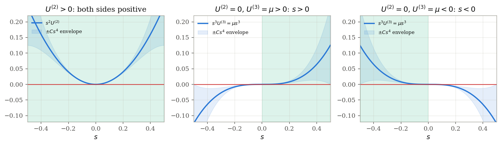
The first figure illustrates the mechanism of the abstract framework: the infimum $U(x,s)=s^2{U}^{(2)}+s^3{U}^{(3)}+O(s^4)$ with the $O(s^4)$ envelope shaded. Away from the degeneracy locus the parabolic term $s^2{U}^{(2)}$ dominates and both small directions $s>0$, $s<0$ are positive; on the degeneracy locus the parabolic term vanishes and the cubic term $s^3\mu$ decides the direction — positive for $s>0$ when $\mu >0$, for $s<0$ when $\mu <0$ — with the green window showing where the cubic dominates the envelope.

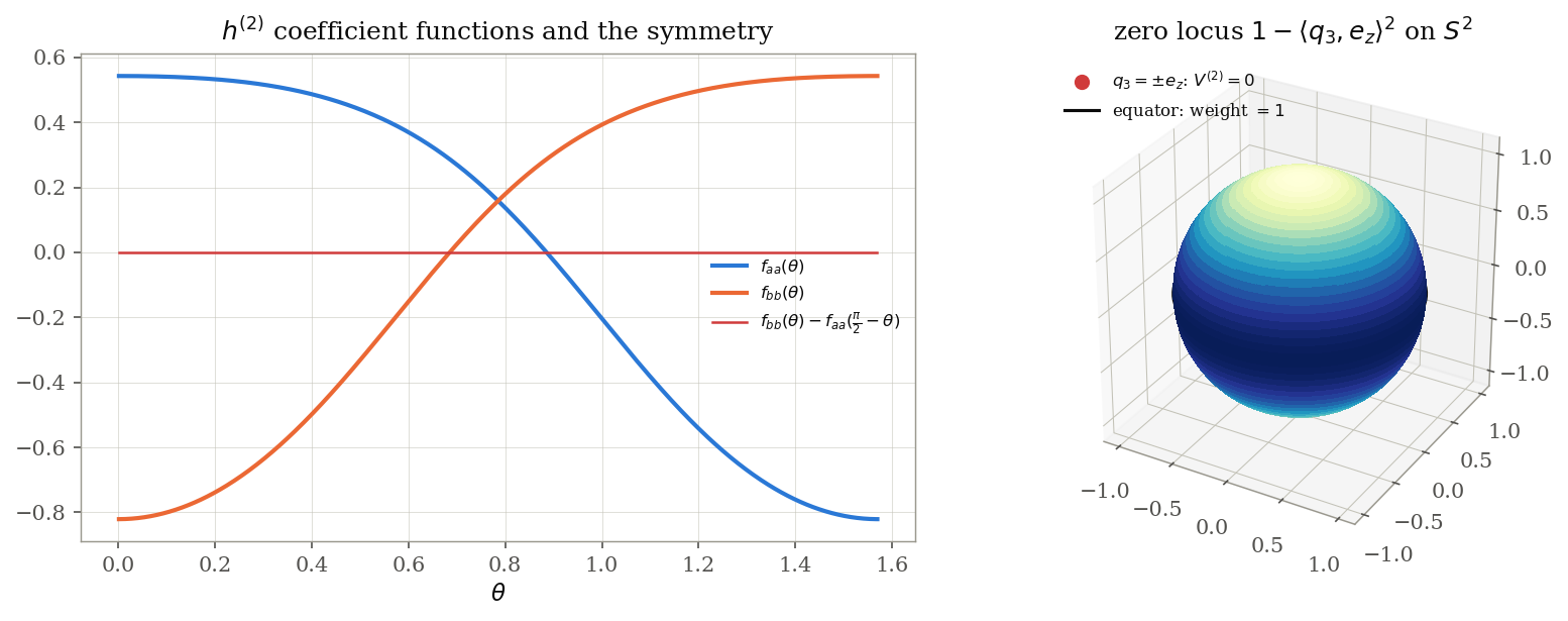
The second figure records two checks on the data of the ansatz: the coefficient functions $f_{aa},f_{bb}$ of $h_{aa}^{(2)},h_{bb}^{(2)}$, together with the residual of the symmetry $f_{bb}(\theta )=f_{aa}(\frac{\pi }{2}-\theta )$ (the red curve, machine zero), and the zero locus of the weight $1-⟨q_3,e_z{⟩}^2$ on the sphere of values of $q_3$ — it vanishes exactly at the poles $q_3=\pm e_z$, which are the points of the critical torus $\Sigma$, and is maximal (value $1$) on the equator, where $V^{(2)}\ge \delta$ holds.

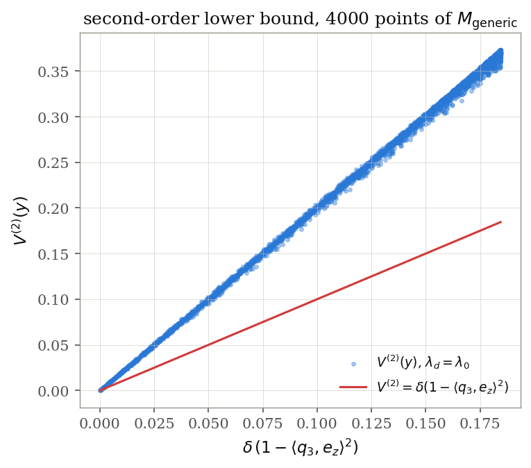
The third figure plots $V^{(2)}(y)$ against $\delta (1-⟨q_3,e_z{⟩}^2)$ for $4000$ random points of $M_{\mathrm{generic}}$ at the admissible value ${\lambda }_d=\frac{3}{4}\sqrt{c_0}$; every point lies on or above the diagonal, confirming the second-order lower bound of the framework.

The script deliberately does not re-derive the ten $V^{(2)}$ identities or the integral identity ${\pi }^2/(18\sqrt{3})$ — those are the content of the companion Mathematica notebook and remain the single point at which the proof depends on external computation. What the script does establish is that everything else in the proof chain is exact: given those identities, the positivity theorem follows by verified, purely structural steps.

Links

• on min-max theory and the Willmore conjecture — Marques–Neves’s min-max resolution of the Willmore conjecture is another landmark in the variational study of curvature-driven geometric existence questions, and the closest analogue in this archive to the strategy of deforming a known configuration into a strictly curved one.
• on curvature-dimension geometry of metric measure spaces — the curvature-dimension condition $CD(K,N)$ provides the synthetic, metric-measure-theoretic counterpart of sectional curvature lower bounds; the Cheeger–Müter metric’s quantitative gap $\sigma d(\cdot ,\mathcal{Z}{)}^2$ is the smooth prototype of the comparison statements used there.

📚 References

🐻  Bourguignon, J.-P. 1975. Some constructions related to H. Hopf’s conjecture on product manifolds. In Differential geometry (Proc. Sympos. Pure Math., Vol. XXVII, Stanford Univ., Stanford, Calif., 1973, Part 1), pp. 33–37. , American Mathematical Society.

🐻  Bourguignon, J.-P., Deschamps, A. & Sentenac, P. 1972. Conjecture de H. Hopf sur les produits de variétés. Annales Scientifiques de l’École Normale Supérieure 5, 277–302.

🐻  Brendle, S. & Hung, P.-K. 2026. A metric on S²\times S² with positive sectional curvature.

🐻  Cheeger, J. 1973. Some examples of manifolds of nonnegative curvature. Journal of Differential Geometry 8, 623–628.

🐻  Gromoll, D. & Meyer, W. 1974. An exotic sphere with nonnegative sectional curvature. Annals of Mathematics 100(2), 401–406.

🐻  Hamilton, R.S. 1982. Three-manifolds with positive Ricci curvature. Journal of Differential Geometry 17, 255–306.

🐻  Hsiang, W.-Y. & Kleiner, B. 1989. On the topology of positively curved 4-manifolds with symmetry. Journal of Differential Geometry 29, 615–621.

🐻  Müter, M. 1987. Krümmungserhöhende Deformationen mittels Gruppenaktionen. phdthesis. Universität Münster,p.

🐻  Petersen, P. & Wilhelm, F. 2008. An exotic sphere with positive sectional curvature.

🐻  Ziller, W. 2009. On M. Müter’s Ph.D. thesis on Cheeger deformations.