Sharp one-third stability of Brenier maps

Source and verification

This article explains family 374 of the October 6, 2026 OpenAI collection. Research conclusions are attributed to its manuscripts. The review covers statements, introductions, and selected proof mechanisms; it is not an independent verification of the complete proofs.

Overview

A small displacement of a target measure can reassign a much larger portion of the source under optimal transport. Family 374 claims a sharp one-third Hölder estimate for Brenier maps with a uniform convex source. A three-atom example makes the obstruction to better exponents explicit.

🏷️ Preliminaries: quadratic maps and Wasserstein distance

Let $K\subset {\mathbb{R}}^d$ be a compact convex body with interior, and let $\rho =|K{|}^{-1}{1}_{K}dx$. For a target probability measure $\mu$, the quadratic optimal map $T_{\mu }$ minimizes $\int |x-T(x){|}^{2}d\rho$ subject to $T_{\#}\rho =\mu$. It is unique up to a source-null set and is the gradient of a convex potential.

The distance between target measures is

$$\begin{array}{c}{W}_2(\mu ,\nu {)}^2\\ =\underset{\pi \in \Pi (\mu ,\nu )}{\inf }\int |y-z{|}^{2}d\pi (y,z).\end{array}$$

This allows the best coupling of the targets. In contrast, $\Vert T_{\mu }-T_{\nu }{\Vert }_{L^2(\rho )}$ compares the two images of each fixed source point. That coupling need not be optimal between the targets. Indeed $W_2(\mu ,\nu )\le \Vert T_{\mu }-T_{\nu }{\Vert }_2$; an upper bound in the reverse direction is the nontrivial stability question.

🏷️ The claimed uniform estimate

Family 374, as stated in the manuscript

For $d\ge 2$ and every fixed nonempty compact target container $Y$, there is $C(K,Y)<\infty$ such that

$$\begin{array}{c}\Vert T_{\mu }-T_{\nu }{\Vert }_{L^2(\rho )}\\ \le C(K,Y)W_2(\mu ,\nu {)}^{1/3}\end{array}$$

for all targets supported in $Y$. No larger exponent works uniformly, even on a fixed cube with three-atom targets. (OpenAI, 2026)

Atomic masses may become small and sites may approach one another. The constant does not depend on a nondegeneracy condition for the targets. More regular target classes can have stronger estimates with constants depending on that extra regularity.

🏷️ A worked sharpness example

Take $K=Y=[-1,1{]}^d$, $0<a<1/2$, and $b=a/2$. Consider convex potentials

$$\begin{array}{rl}{u}_a(x)& =\max \{-x_1,x_1,a\},\\ {\tilde{u}}_a(x)& =\max \{-x_1,x_1,a+b{x}_2\}.\end{array}$$

Their gradients are optimal maps to their own pushforward measures. This follows directly from the supporting inequalities for the affine maxima: maximizing $\int x\cdot y$ is equivalent to minimizing quadratic cost when the marginals are fixed.

The first central cell is $A=\{|x_1|<a\}$, where the gradient is zero. The second is $B=\{|x_1|<a+b{x}_2\}$, where it is $b{e}_2$. Both cells have mass $a$; the outer slopes remain $\pm e_1$ with equal masses $(1-a)/2$.

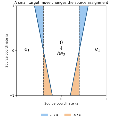
The figure uses $a=2/5$ and $b=1/5$. Dashed lines bound the original central cell $A$; solid lines bound the tilted cell $B$. Shaded regions switch between central and outer slopes. Labels are map values, not points plotted in target space. The remaining source coordinates integrate out.

The targets therefore differ only by moving mass $a$ from $0$ to $b{e}_2$. This coupling is optimal because the second coordinate alone forces its full cost, giving $W_2^2=a{b}^2$.

At a slice $x_2=t$, the symmetric difference of the central cells has probability $b|t|$. Averaging gives $\rho (A△B)=b/2$. On this set the maps switch between central and outer slopes, producing an order-one first-coordinate change. Orthogonality of coordinates yields

$$\begin{array}{rl}\Vert T_{{\mu }_a}-T_{{\nu }_a}{\Vert }_2^2& =b/2+a{b}^2,\\ W_2({\mu }_a,{\nu }_a)& =a^{3/2}/2,\\ \Vert T_{{\mu }_a}-T_{{\nu }_a}{\Vert }_2& =\frac{1}{2}\sqrt{a}\sqrt{1+a^2}.\end{array}$$

For an exponent $\alpha >1/3$, the ratio of the last quantity to $W_2^{\alpha }$ diverges like $a^{(1-3\alpha )/2}$. This elementary construction explains why even a square-root estimate fails in the uniform class.

🏷️ The proposed matching upper bound

For finite targets, a convex potential is a maximum of affine functions; its cells have prescribed masses. Moving intercepts changes both cell masses and first moments. The manuscript’s central estimate controls the squared first-moment derivatives, weighted by inverse cell masses, by the similarly weighted mass derivatives, uniformly through cell degeneration.

Along a transport of target sites, the mass constraints give a graph-Laplacian equation for intercept velocities. The moment estimate controls the needed velocities without a uniform bound for the inverse graph Laplacian. After fixing the additive constants of the potentials, this produces an $L^2$ potential difference of order $W_2$.

A convex-gradient interpolation estimate then has the form

$$\begin{array}{c}\Vert \nabla u-\nabla v{\Vert }_2^2\\ \le C(h^{-2}\Vert u-v{\Vert }_2^2+h).\end{array}$$

Balancing terms with $h=W_2^{2/3}$ gives a squared-gradient bound of order $W_2^{2/3}$ and hence the one-third exponent. Approximation extends the finite-target result to arbitrary compactly supported targets. The uniform moment estimate is the main new input; the balancing calculation alone does not establish it.

🏷️ Key steps and proof outlines

The crucial estimate concerns cell moments, not site separation

For a finite target, write the convex potential as $u(x)={\max }_i\{x\cdot y_i+c_i\}$. Its cells $P_i$ are the regions where the $i$th affine function wins. Let $M_i=\rho (P_i)$ and $B_i={\int }_{P_i}xd\rho$. Varying the intercepts in a direction $q$ while keeping the sites fixed gives the source’s central estimate

$$\sum _i\frac{|D{B}_i[q]{|}^2}{M_i}\le 162R^2\sum _i\frac{|D{M}_i[q]{|}^2}{M_i},$$

where $K\subset B(0,R)$ and $\rho$ is normalized volume on $K$. The bound is uniform even when some masses or site separations are tiny.

Proof outline. Compare the cells at $c-sq$ and $c+sq$. Couple their uniform laws by the same successive conditional quantiles. The midpoint of the coupled points belongs to the original cell: averaging the two affine cell inequalities cancels the intercept perturbation. The triangular quantile maps have products of diagonal derivatives equal to their cell volumes. Arithmetic–geometric mean applied to those derivatives bounds the midpoint density by the inverse geometric mean of the two volumes.

Now use $\Phi (x)=R^2-|x{|}^2\ge 0$ and its exact midpoint identity

$$\Phi \left(\frac{X+Z}{2}\right)=\frac{\Phi (X)+\Phi (Z)}{2}+\frac{|X-Z{|}^2}{4}.$$

Summing over cells cancels the endpoint partition integrals. If ${\alpha }_i,{\beta }_i$ are the two masses and ${\gamma }_i=\sqrt{{\alpha }_i{\beta }_i}$, the remaining estimate controls ${\sum }_i{\gamma }_i\mathbb{E}|X_i-Z_i{|}^2$ by $5R^2{\sum }_i({\alpha }_i-{\beta }_i{)}^2/{\gamma }_i$. First moments differ by a mass-change term plus a displacement term. Cauchy–Schwarz bounds both; division by $(2s{)}^2$ and passage to the derivative limit give the displayed constant. The allowed size of $s$ may depend on the configuration, but the resulting derivative constant does not. (OpenAI, 2026)

Moving sites while holding their transported masses fixed

Take an optimal finite coupling ${\sum }_i{m}_i{\delta }_{(y_i^0,y_i^1)}$ between the targets and interpolate $y_i(t)=(1-t)y_i^0+t{y}_i^1$. Put $v_i=y_i^1-y_i^0$ and $w=W_2(\mu ,\nu )$, so ${\sum }_i{m}_i|v_i{|}^2=w^2$. Pairwise optimality gives $(y_i^0-y_j^0)\cdot (y_i^1-y_j^1)\ge 0$; hence distinct endpoint pairs produce distinct sites at every interior time.

Choose intercepts so the cell masses remain $m_i$, normalized by ${\sum }_i{m}_i{c}_i(t)=0$. Their derivatives $r_i=c_i^{\prime }(t)$ have weighted mean zero. The cell-mass derivative matrix is a connected weighted graph Laplacian, so an intercept direction $q$ can be chosen with $D{M}_i[q]=m_i{r}_i$. Differentiating the fixed-mass constraints and using symmetry of face contributions yields

$$\sum _i{m}_i{r}_i^2=-\sum _i{v}_i\cdot D{B}_i[q].$$

Weighted Cauchy–Schwarz and the moment estimate give

$${\left(\sum _i{m}_i{r}_i^2\right)}^{1/2}\le \sqrt{162}Rw.$$

No bound on $q$ itself is required. Since ${\partial }_t{u}_t=x\cdot v_i+r_i$ on cell $i$, integration in time proves $\Vert u_1-u_0{\Vert }_{L^2(\rho )}\le (1+\sqrt{162})Rw$. This is the stable quantity before taking gradients. (OpenAI, 2026)

Why differentiation changes a linear estimate into a one-third estimate

On each coordinate interval of the convex body, a convex $L$-Lipschitz function has a monotone derivative bounded by $L$. Its forward difference quotient differs from that derivative by a nonnegative quantity whose integral is at most $2Lh$: the interior translated integrals cancel, leaving two endpoint intervals of length $h$. Squaring costs another factor $2L$. The excluded boundary portions also have total volume bounded by $h$ times the coordinate projection area.

Summing these slice estimates gives, for $f=u_0-u_1$,

$$\Vert \nabla u_0-\nabla u_1{\Vert }_2^2\le \frac{12d}{h^2}\Vert f{\Vert }_2^2+\frac{28L^2{P}_K}{|K|}h,$$

where $P_K$ is the sum of coordinate projection volumes. Substituting $\Vert f{\Vert }_2=O(w)$ and choosing $h=w^{2/3}$ balances the two terms at order $w^{2/3}$. Taking square roots yields the exponent $1/3$.

Finally, approximate arbitrary compactly supported targets by finite nets. The uniform estimate makes their maps Cauchy in $L^2$. Uniform limits of normalized convex potentials provide supporting inequalities for the limit map; the Fenchel equality identifies it as the unique optimal map. Thus no lower target-density bound or uniform atom separation is introduced in the limiting argument. (OpenAI, 2026)

See Also

• Family 373 shows why deterministic optimal maps need not exist for a different multi-marginal cost.
• Family 368 also separates convergence of maps from convergence of their derivatives.

🏷️ Manuscripts and verification scope

• Sharp One-Third Stability of Brenier Maps — pinned manuscript and companion source.

The family scope page describes selected formalization coverage. The scope page describes both the uniform one-third estimate and the obstruction to every larger exponent using three-atom targets on a fixed cube. No Lean build, axiom audit, or manuscript-to-formal-statement equivalence check was performed for these notes.

OpenAI collection provides prerequisites and the reading sequence; coverage register records completed and pending families.

🐻  OpenAI 2026. Sharp One-Third Stability of Brenier Maps.