No conjugate points without nonpositive curvature: a three-manifold and its geodesic neck

Source and verification

This article explains family 358 of the October 6, 2026 OpenAI collection. Research conclusions are attributed to its manuscripts. The review covers statements, introductions, and selected proof mechanisms; it is not an independent verification of the complete proofs.

🏷️ Jacobi fields and the distinction between two existence questions

Let $\gamma$ be a unit-speed geodesic on a smooth Riemannian manifold, and write $T=\dot{\gamma }$. A Jacobi field is a vector field satisfying

$$D_s^{2}J+R(J,T)T=0.$$

Here $D_s$ denotes covariant differentiation along the geodesic, and $R$ is the curvature tensor. Jacobi fields describe the infinitesimal separation of nearby geodesics. Two points along $\gamma$ are conjugate when a nonzero Jacobi field vanishes at both of their parameter values.

Nonpositive sectional curvature prevents this kind of refocusing. For a variation field $V$, the relevant quadratic expression is the index form

$$\begin{array}{rl}{I}_J(V)=& {\int }_J|D_{s}V{|}^{2}ds\\ & -{\int }_J⟨R(V,T)T,V⟩ds.\end{array}$$

With the convention used here, the curvature term is nonpositive when sectional curvature is nonpositive. The integrand is then nonnegative.

A metric without conjugate points can nevertheless have positive sectional curvature in some regions. That does not answer a different question: might its underlying manifold admit some other nonpositively curved metric? Family 358 constructs a manifold for which the answer is negative. (OpenAI, 2026)

The manuscript's existence theorem

There is a closed, connected, orientable smooth three-manifold with a smooth Riemannian metric without conjugate points, although the same manifold admits no smooth Riemannian metric of everywhere nonpositive sectional curvature.

“Closed” means compact without boundary. Compactness makes every smooth Riemannian metric on the manifold complete, so geodesics extend for all time. The two assertions of the theorem require different arguments: a topological obstruction excludes all nonpositively curved metrics, while an explicit construction supplies one metric without conjugate points.

For comparison, a metric has no focal points if every nonzero normal Jacobi field starting at zero satisfies $\frac{d}{ds}|J(s){|}^2>0$ for positive time. This is stronger than absence of conjugate points. The manuscript also deduces a no-focal-points obstruction from an imported equivalence specific to closed three-manifolds; that consequence is separate from the main construction.

🏷️ Two product pieces with incompatible boundary geometry

Take a compact torus with one disk removed, denoted $\Sigma$, and form two copies of $\Sigma \times S^1$. Each has a torus boundary. On the $i$th boundary, let $h_i$ be the surface-boundary loop and $f_i$ the circle-factor loop. Glue the boundaries using

$$h_2=h_1+f_1,f_2=h_1.$$

The integer matrix has determinant $-1$, so it reverses boundary orientation and produces a closed orientable three-manifold. Insert a cylinder $[0,1]\times T^2$ between the pieces; inserting this collar does not change the smooth manifold.

The geometric obstruction can be summarized in a Euclidean plane. Under a hypothetical nonpositively curved metric, the common torus determines two independent translation vectors $u,v$. The product structure of the first piece forces $u\perp v$. The second product structure forces the translations corresponding to $h_2,f_2$ to be perpendicular, giving

$$0=⟨u+v,u⟩=|u{|}^2.$$

This contradicts $u\ne 0$.

The perpendicularity is an imported geometric constraint, not an arbitrary requirement that the constructed boundary metric be rectangular. The source derives it through the flat torus theorem: the circle direction gives a line factor, and the surface boundary has zero translation along that factor. Both constraints hold in the same invariant Euclidean plane. This explains why the obstruction applies to every candidate nonpositively curved metric, rather than merely to product metrics on the chosen pieces. The manuscript gives the fuller covering-space argument and a stronger obstruction to locally CAT(0) metrics. (OpenAI, 2026)

The rest of the article develops the differential-geometric construction and its variational estimates.

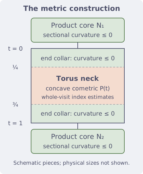
The diagram separates the regions where curvature directly controls the index form from the neck region requiring an estimate over each entire visit. It does not depict the manifold as an embedded subset of Euclidean space.

🏷️ A concave inverse metric on the connecting neck

Write the neck metric as

$$\begin{array}{c}g=d{t}^2+d{x}^{T}Q(t)dx,\\ P(t)=Q(t{)}^{-1}.\end{array}$$

The two torus coordinates are locally lifted to ${\mathbb{R}}^2$. The positive definite matrix $Q$ measures lengths of torus tangent vectors; its inverse $P$ is called the cometric. The construction makes $P$ concave in the matrix sense:

$$-P^{\prime \prime }(t)⪰0.$$

This means $b^T(-P^{\prime \prime })b\ge 0$ for every vector $b$. It will make a completed-square expression for the coordinate second variation nonnegative. It does not assert nonpositive sectional curvature throughout the neck.

Here is the explicit choice. Define

$$\begin{array}{c}a(u)=\{\begin{array}{ll}{e}^{-1/(2/3-u)},& u<2/3,\\ 0,& u\ge 2/3,\end{array}\\ A(u)={\int }_0^{u}a(y)dy.\end{array}$$

Choose a fixed smooth nondecreasing cutoff $\chi$, zero up to $5/12$ and one from $7/12$ onward. For a small positive parameter $\delta$, put

$$\begin{array}{rl}ϵ& ={\delta }^2,H=e_2+ϵ\chi (t)e_1,\\ d_1(t)& =1+\delta A(t),\\ d_2(t)& =1+\delta A(1-t),\\ P(t)& =d_1(t)e_1{e}_1^T+d_2(t)H{H}^T.\end{array}$$

The diagonal concavity has size $\delta$, whereas the moving-frame perturbation has size ${\delta }^2$. The frame changes only where both diagonal second derivatives are strictly negative. For sufficiently small $\delta$, this yields uniform positive-definiteness and

$$|P^{\prime }p{|}^2\le C\delta p^T(-P^{\prime \prime })p$$

in either endpoint frame. This stronger derivative estimate will control a mixed term in the returning-geodesic argument, including directions where $-P^{\prime \prime }$ is singular.

The coordinate shear can be tiny while the topological gluing remains fixed. Choose periods $B_1=ϵB_2$. The right endpoint frame is $(e_2+ϵe_1,e_1)$, with periods $(B_2,B_1)$. Its surface-boundary period vector is exactly

$$B_2(e_2+ϵe_1)=B_1{e}_1+B_2{e}_2.$$

Thus it realizes $h_2=h_1+f_1$ for every positive $ϵ$.

At either end use the inward coordinate $\tau$, equal to $t$ on the left and $1-t$ on the right. In its endpoint frame the cometric is exactly

$$\begin{array}{c}{P}_i(\tau )=\left(\begin{array}{cc}1+\delta A(\tau )& 0\\ 0& b\end{array}\right),\\ b=1+\delta A(1),\end{array}$$

for $0\le \tau \le 1/4$. The surface factor has warping function ${\ell }_0=(1+\delta A{)}^{-1/2}$, with ${\ell }_0^{\prime \prime }\ge 0$, so its Gaussian curvature $-{\ell }_0^{\prime \prime }/{\ell }_0$ is nonpositive.

To attach the compact pieces smoothly, the source extends this warping function through a strictly convex collar to an exact exponential cusp profile. Truncating a hyperbolic punctured torus at a sufficiently short horocycle supplies the compact core. The formulas agree on whole neighborhoods of the seams, giving a smooth metric rather than only finite-order matching. The periods are chosen after $\delta$, so fitting the cusps does not change any estimate on the lifted neck. (OpenAI, 2026)

🏷️ Geodesic energy and the endpoint correction

Translation invariance in $x$ gives a conserved torus momentum

$$\begin{array}{c}p=Q(t)\dot{x},F(t)=p^{T}P(t)p,\\ v=\dot{t},v^2=1-F(t),\\ \dot{v}=-\frac{1}{2}{F}^{\prime }(t).\end{array}$$

Since $P$ is concave, so is $F$. These equations classify visits to the open neck. A visit either stays at a constant interior height for all time, crosses monotonically between the two boundaries, approaches an interior equilibrium on a half-infinite interval, or turns once and returns to its entry boundary. Finite entry and exit times are transverse. A geodesic tangent to a boundary either stays in that boundary or locally lies outside the open neck.

For a field $V=(w,z)$, where $w$ is the interval component and $z$ the torus component, define

$$\begin{array}{rl}E(V)=\int (& {\dot{w}}^2+|\dot{z}-P^{\prime }pw{|}_Q^2\\ & -\frac{1}{2}{F}^{\prime \prime }(t)w^2)ds.\end{array}$$

Every term is nonnegative. Direct differentiation of the energy of the coordinate-linear variation produces this expression: the identities for differentiating $Q=P^{-1}$ complete the square. But the intrinsic index form is

$$\begin{array}{rl}{I}_{[a,c]}(V)=& E_{[a,c]}(V)\\ & -[⟨T,\Gamma (V,V)⟩{]}_a^c,\end{array}$$

where $\Gamma$ denotes the Christoffel symbols in these coordinates. The coordinate-linear variation has covariant acceleration $\Gamma (V,V)$, which accounts for the boundary correction. Dropping it would not prove the required passage estimate.

Remove the tangential energy by defining

$$\begin{array}{rl}{q}_V& =⟨V,T⟩,\\ I_J^{\perp }(V)& =I_J(V)-{\int }_J|{\dot{q}}_V{|}^{2}ds.\end{array}$$

This is precisely the index form of the normal component of $V$. Consequently it is unchanged under $V\mapsto V+hT$, with arbitrary smooth $h$, even when $h$ does not vanish at passage endpoints.

For a monotone passage, take $h=-w/v$ to make the interval component zero. The boundary correction then has a favorable sign, and Cauchy–Schwarz in the $Q$ metric gives

$$|\dot{z}{|}_Q^2-|p^T\dot{z}{|}^2\ge (1-F)|\dot{z}{|}_Q^2\ge 0.$$

If $v$ tends to zero at an infinite endpoint, this division causes no problem: the original compactly supported field already vanishes beyond some finite time. No uniform bound on $1/|v|$ is needed. Constant-height visits are handled by taking the normal field and placing integration endpoints outside its support. Returns entirely inside an endpoint collar use the pointwise nonpositive-curvature estimate. (OpenAI, 2026)

🏷️ A returning excursion and its positive boundary term

For a remaining return, choose inward coordinates at its entry boundary and write its time interval as $[0,L]$. It has one turn at $L/2$, with

$$\begin{array}{c}t(0)=t(L)=0,\\ t(L/2)=t_{\ast }>1/4,\\ v(0)=-v(L)=v_0>0.\end{array}$$

Set $e=(1,0{)}^T$ and $\kappa =\delta a(0)$. Concavity and the endpoint formula give

$$\begin{array}{c}0<F^{\prime }(t)\le \kappa p_1^2,\\ 0<v_0^2\le \kappa p_1^2,p_1\ne 0.\end{array}$$

A single tangential adjustment can simultaneously make $w(0)=w(L)=0$ and $q_V$ affine. Indeed, prescribe the adjustment’s endpoint values to cancel $w$, then interpolate the resulting endpoint values of $q_V$ affinely and subtract the old $q_V$. This uses no restriction on the original variation field’s endpoint values.

Let $X=z(L)-z(0)$ and $\mu =\kappa v_0/4$. The intrinsic formula gives

$$\begin{array}{rl}{I}^{\perp }(V)\ge & E(V)+\mu (e^{T}X{)}^2\\ & -\frac{(p^{T}X{)}^2}{L}.\end{array}$$

The positive term comes from the two boundary values of $z_1$: their contribution is $\kappa v_0(z_1(0{)}^2+z_1(L{)}^2)/2$, and the sum of squares controls half the square of their difference. The last term is the energy of the affine tangential component.

The task is therefore to show that the coordinate energy, supplemented by a penalty on one component of $X$, controls $p^{T}X$. This is where the shape of the entire excursion enters.

🏷️ Timing estimates and quadratic optimization

On the first half of a returning visit,

$$\ddot{v}=-\frac{1}{2}{F}^{\prime \prime }(t)v\ge 0.$$

Thus $v$ lies below the chord from $v_0$ to zero. Reflection across the turn gives

$${\int }_0^L{v}^{2}ds\le \frac{L{v}_0^2}{3}.$$

Since the turn leaves the endpoint collar, concavity of $t(s)$ puts $t\ge 1/8$ throughout the middle half of the excursion. On that half the derivative $F^{\prime }$ has dropped by the fixed factor $a(1/8)/a(0)=e^{-9/26}$. Integrating $\dot{v}=-F^{\prime }/2$ therefore gives the strict margin

$$\begin{array}{c}4v_0\le \beta \kappa p_1^{2}L,\\ \beta =\frac{1+e^{-9/26}}{2}<1.\end{array}$$

This uses no upper bound on $L$.

For the energy estimate, set $\xi =\dot{z}-P^{\prime }pw$ and give $H_0^1(0,L)$ the norm

$$\Vert w{\Vert }_{\mathcal{D}}^2={\int }_0^L\left({\dot{w}}^2-\frac{1}{2}{F}^{\prime \prime }{w}^2\right)ds.$$

For a constant covector $q$, define ${\Phi }_q(w)={\int }_0^L{q}^T{P}^{\prime }pwds$. Integrating $\dot{z}$ expresses $q^{T}X$ as a linear functional of $(\xi ,w)$ in the Hilbert direct sum whose squared norm is $E$. Its squared dual norm is the positive quadratic form

$$S(q,q)={\int }_0^L{q}^{T}Pqds+\Vert {\Phi }_q{\Vert }_{{\mathcal{D}}^{\ast }}^2.$$

Cauchy–Schwarz gives $|q^{T}X{|}^2\le S(q,q)E$. Split $p=(p-\alpha e)+\alpha e$ and include the boundary penalty. A second Cauchy–Schwarz inequality shows that

$$|p^{T}X{|}^2\le C(\alpha )(E+\mu (e^{T}X{)}^2),$$

where

$$\begin{array}{rl}C(\alpha )& =S(p-\alpha e,p-\alpha e)\\ & +{\alpha }^2/\mu ,\\ \underset{\alpha }{\min }C(\alpha )& =S(p,p)\\ & -\frac{S(p,e{)}^2}{S(e,e)+{\mu }^{-1}}.\end{array}$$

The proof needs this minimum to be at most $L$. Its estimates are

$$\begin{array}{rl}S(p,p)& \le L(1+v_0^2),\\ S(e,e)& \le C_{e}L,\\ |S(p,e)-L{p}_1|& \le C_m\delta L|p_1|.\end{array}$$

The first bound uses ${\Phi }_p(w)=2\int v\dot{w}$ and the chord estimate. The second uses the derivative domination $|P^{\prime }p{|}^2\le C\delta (-F^{\prime \prime })$. For the mixed bound, positivity of $P^{\prime }(0)-P^{\prime }(t)$ controls its pairing with $e,p$ by its two diagonal quadratic forms. This retains the factor $|p_1|$. Replacing it by $|p|$ would lose uniformity for nearly tangential incidence.

Put $r=v_0^2/p_1^2$. Then $r\le a(0)\delta$, while the timing margin implies $L\mu \ge r/\beta$. Combining the preceding inequalities gives

$$\frac{S(p,e{)}^2}{S(e,e)+{\mu }^{-1}}\ge L{v}_0^2\frac{(1-C_m\delta {)}^2}{\beta +C_{e}a(0)\delta }.$$

For one sufficiently small positive $\delta$, the last fraction is at least one, because $\beta <1$. The boundary correction therefore removes the entire possible excess $L{v}_0^2$ in $S(p,p)$. This proves $I^{\perp }(V)\ge 0$ for every returning passage.

The parameter choice depends only on the fixed construction constants, not on $L,v_0,p_1$, or the turning height. Hence one metric handles arbitrarily long returns and arbitrarily shallow incidence, through either endpoint. (OpenAI, 2026)

🏷️ From passage estimates to absence of conjugate points

For a compactly supported field on a complete geodesic, the original intrinsic index integrand is continuous and absolutely integrable. Visits to the open neck are a countable disjoint collection of intervals. Every whole-visit integral is nonnegative by the passage estimates; on the complement, sectional curvature is nonpositive and the integrand is pointwise nonnegative. Countable additivity therefore gives

$$I_{\mathbb{R}}(V)\ge 0.$$

This includes infinitely many visits with accumulating endpoints. Tangential adjustments chosen on different visits need not match, because the sum uses the unchanged intrinsic normal index of the original field. Times spent on interfaces are included in the complement, even if they form a set of positive measure.

Finally, suppose a nonzero Jacobi field $J$ vanishes at $a<b$. Extend it by zero outside $[a,b]$ to obtain a compactly supported $H^1$ field $\hat{J}$. Integration by parts gives $I(\hat{J})=0$. Smooth approximation extends the proved nonnegativity to such $H^1$ fields.

Let $B$ be the symmetric bilinear form associated with $I$. For every smooth compactly supported $W$ and every real $t$,

$$\begin{array}{rl}0\le & I(\hat{J}+tW)\\ =& 2tB(\hat{J},W)+t^{2}I(W).\end{array}$$

Both signs of small $t$ force $B(\hat{J},W)=0$. But integration by parts gives the endpoint derivative jump. Choose $W$ supported near $a$, with $W(a)=D_{s}J(a)$, to obtain

$$B(\hat{J},W)=-|D_{s}J(a){|}^2<0.$$

The strict inequality follows from uniqueness for the Jacobi equation: zero value and zero derivative at $a$ would force $J$ to vanish identically. This contradiction proves the no-conjugate-points conclusion. Constant geodesics cause no exception, since their Jacobi equation is the ordinary equation $J^{\prime \prime }=0$.

🏷️ Key steps and proof outlines

The mixed estimate retains the small incidence parameter

The estimate for $S(p,e)$ deserves a separate argument because nearly tangential returns can have $|p_1|\ll |p|$. Set $D(t)=P^{\prime }(0)-P^{\prime }(t)$. Matrix concavity gives $D(t)⪰0$, while the returning-geodesic equations give

$$0\le p^{T}D(t)p\le \kappa p_1^2,e^{T}D(t)e\le C\delta .$$

Cauchy–Schwarz for this positive semidefinite quadratic form, valid even when it is singular, therefore yields

$$|e^{T}D(t)p{|}^2\le C\delta \kappa p_1^2.$$

Since $\kappa =\delta a(0)$, the error has size $\delta |p_1|$. Integrate first in height, using $e^{T}P(0)p=p_1$, and then over the passage to obtain an error $O(\delta L|p_1|)$. The other part of $S(p,e)$ is the dual pairing of ${\Phi }_p$ and ${\Phi }_e$. Its bounds are respectively $O(\sqrt{L}{v}_0)$ and $O(\sqrt{\delta L})$; the inequality $v_0^2\le \delta a(0)p_1^2$ gives the same error. This explains why the quadratic optimization remains valid uniformly as the incidence angle tends to zero.

Local gauges need not join across the interfaces

The passage proofs change $V$ by different tangential fields on different visits. These auxiliary fields need not define a smooth global field. The quantity being estimated is nevertheless the original intrinsic normal index form, unchanged by every such adjustment.

To assemble the estimates, write the open set of visiting times as disjoint intervals $J_j$. The original index integrand $i_V$ is continuous with compact support, so

$$\sum _j\left|{\int }_{J_j}{i}_{V}ds\right|\le {\int }_{\mathbb{R}}|i_V|ds<\infty .$$

Thus countable additivity applies even if infinitely many visits accumulate. On the complementary times, including time spent on an interface, nonpositive curvature makes the original integrand nonnegative. This avoids an unjustified finite-passage assumption or any need to control the sizes of all auxiliary gauges.

Why a zero index Jacobi field still leads to a contradiction

A Jacobi field $J$ with $J(a)=J(b)=0$ has zero index on $[a,b]$, rather than immediately negative index. Extend it by zero to an $H^1$ field $\hat{J}$; smooth approximation extends index nonnegativity to this field. Let $B$ denote the bilinear index form. Nonnegativity for both signs of $t$ in

$$I(\hat{J}+tW)=2tB(\hat{J},W)+t^{2}I(W)$$

forces $B(\hat{J},W)=0$. Integration by parts instead gives a boundary derivative jump. Choose $W$ supported near $a$, with $W(a)=D_{s}J(a)$, and obtain

$$B(\hat{J},W)=-|D_{s}J(a){|}^2<0.$$

The strict sign follows from uniqueness for the Jacobi equation: both $J(a)$ and $D_{s}J(a)$ cannot vanish for a nonzero solution. These are the final functional-analytic and variational steps in “Uniform control of returning geodesics” and “From passages to absence of conjugate points.” (OpenAI, 2026)

🏷️ Connections and verification scope

The Cartan–Hadamard family develops consequences of nonpositive curvature. This construction separates that curvature hypothesis from the weaker absence of geodesic refocusing. The distributional-curvature family also uses an index-form mechanism, there to recover distance comparison from a lower curvature bound.

The source review read the manuscript’s main file, seven sections including its appendix, and construction figure. The post checks the gluing convention, cometric scaling, endpoint signs, whole-return optimization, timing margin, and countable assembly. It summarizes the topological obstruction geometrically and does not develop its group-theoretic machinery. The cited geometric theorems and the complete research result have not been independently verified.

🏷️ Manuscripts and verification scope

• A Three-Manifold Without Conjugate Points and Without a Nonpositively Curved Metric — pinned manuscript and companion source.

The family scope page describes selected formalization coverage. The documented selection is the main existence theorem, including all geodesics and tangent-bundle Jacobi fields, constant geodesics, and unbounded time intervals. The separate no-focal-points and CAT(0) consequences are outside that documented selection. No Lean build, axiom audit, or manuscript-to-formal-statement equivalence check was performed for these notes.

OpenAI collection provides prerequisites and the reading sequence; coverage register records completed and pending families.

🐻  OpenAI 2026. A Three-Manifold Without Conjugate Points and Without a Nonpositively Curved Metric.