Isoperimetry in the cubic three-torus: balls, tubes, and slabs

Source and verification

This article explains family 354 of the October 6, 2026 OpenAI collection. Research conclusions are attributed to its manuscripts. The review covers statements, introductions, and selected proof mechanisms; it is not an independent verification of the complete proofs.

On a flat three-dimensional torus, a small amount of material can form a ball. More material can wrap around a periodic direction as a solid tube. Near half volume, a slab has only two flat boundary components. This family asks whether any more complicated shape can improve on those three candidates.

The manuscript proves that the candidates exhaust all minimizers in the cubic flat three-torus, including the ties at the two transition volumes. The proof’s distinctive step concerns nested planar sections: individually optimal slices need not fit inside one another, and their required nesting forces an additional area cost. An explicit arithmetic argument closes the resulting one-variable inequality. (OpenAI, 2026)

The prerequisites are multivariable calculus, surface area, the divergence theorem, and elementary variational calculus. We introduce perimeter, curvature conventions, and the stability input before describing the proof. The discussion follows the manuscript’s source; the finite arithmetic checks reproduced below have a narrower scope than the complete geometric theorem.

🏷️ The torus and the perimeter problem

The unit cubic flat torus is ${\mathbb{T}}^3={\mathbb{R}}^3/{\mathbb{Z}}^3$: identify opposite faces of the unit cube, with the Euclidean metric locally. Its total volume is one. A coordinate circle travels once around one periodic direction and has length one.

For a measurable set $E$, its perimeter is the total variation of its indicator function. One definition is

$$P(E)=\underset{|X|\le 1}{\sup }{\int }_E\mathrm{div}Xdx,$$

where the supremum runs over smooth vector fields on the torus. For a smooth region this equals the area of its boundary. The definition also accommodates limits of smooth regions and ignores changes on sets of volume zero.

The isoperimetric profile is

$$I_{\mathrm{unit}}(V)=\inf \{P(E):|E|=V\}.$$

Existence and regularity of minimizers are classical inputs in the manuscript. In dimension three their boundaries are smooth embedded surfaces. Complementation preserves perimeter, so the profile at $V$ equals the profile at $1-V$. It therefore suffices to consider $v=\min (V,1-V)\le 1/2$.

The three candidate calculations are elementary:

Region	Volume	Boundary area
Ball of radius $r$	$4\pi r^3/3$	$4\pi r^2$
Circular tube of radius $r$ around a coordinate circle	$\pi r^2$	$2\pi r$
Coordinate slab of width $w$	$w$	$2$

There are no end caps on a tube: its axis closes periodically. A slab’s two boundary tori each have area one.

Profile and all equality cases

The manuscript proves that $I_{\mathrm{unit}}(V)$ is the minimum of the three expressions

$$(36\pi {)}^{1/3}{v}^{2/3},2\sqrt{\pi v},2.$$

Up to ambient isometry and changes on null sets, all minimizers are balls, circular tubes about shortest closed geodesics, coordinate slabs, and their complements, in the ranges below. (OpenAI, 2026)

Equating consecutive expressions gives

$$V_1=\frac{4\pi }{81},V_2=\frac{1}{\pi }.$$

Smaller volume $v$	Minimizing type	Parameter in the unit torus
$0<v<V_1$	Ball	$r=(3v/(4\pi ){)}^{1/3}$
$V_1<v<V_2$	Tube	$r=\sqrt{v/\pi }$
$V_2<v\le 1/2$	Slab	Width $v$

At $V_1$, both balls and tubes minimize. At $V_2$, both tubes and slabs minimize. The classification excludes additional minimizers at these endpoints. For $V>1/2$, take complements of the listed regions at volume $1-V$.

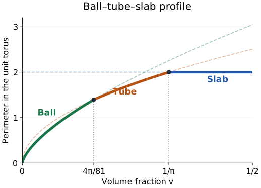
The bold curves form the candidate lower envelope; dashed curves show the competing perimeter formulas. The theorem asserts that the true profile equals this envelope. At the last volume of the ball branch its radius is $1/3$, and at the last volume of the tube branch its radius is $1/\pi$. Both are below the transverse injectivity radius $1/2$, so these branch representatives embed without self-intersection.

A tube around a primitive closed geodesic of length $L\ge 1$ has perimeter $2\sqrt{\pi Lv}$ at enclosed volume $v$. Equality with the tube candidate therefore requires $L=1$. Similarly, parallel planar tori bounding a region have total area at least two, with equality only for a pair of coordinate tori. The cubic metric matters: general flat tori have different shortest lattice vectors and do not fall under this particular formula or classification.

🏷️ Curvature, stability, and the two-volume reduction

The source doubles all lengths and works on $T={\mathbb{R}}^3/(2{\mathbb{Z}}^3)$. It uses normalized volume and area

$$V=\frac{|E|}{8},A=\frac{|\partial E|}{8}.$$

Thus $V$ is still the original volume fraction, while $A$ is half the unit-torus perimeter. The outward sum curvature is $h=k_1+k_2$, positive on a ball. It is measured in the doubled metric and is not divided by eight. The normalized candidate profile is

$$\begin{array}{c}F(V)=\min \{F_b(v),F_t(v),1\},\\ F_b(v)=(9\pi /2{)}^{1/3}{v}^{2/3},\\ F_t(v)=\sqrt{\pi v}.\end{array}$$

A volume-constrained area minimizer has constant $h$. Its second variation is nonnegative for normal speeds of mean zero:

$$\begin{array}{rl}\mathcal{Q}(f,f)& ={\int }_{\Sigma }(|\nabla f{|}^2-|\mathrm{II}{|}^2{f}^2)dS\\ & \ge 0.\end{array}$$

Here $\Sigma =\partial E$, $\mathrm{II}$ is the second fundamental form, and the mean-zero condition is ${\int }_{\Sigma }fdS=0$. It expresses first-order preservation of volume.

The manuscript imports classical structure results of Hauswirth–Pérez–Romon–Ros and Ritoré–Ros. A minimizing boundary is either a union of parallel planar surfaces or is connected. In the connected case, genus zero gives a sphere, genus one gives a planar or circular-cylinder quotient, and genus is at most four. A nonstandard minimizer therefore has genus $g\ge 2$, where genus counts handles, and satisfies

$$h^{2}A\le \pi .$$

For genus two or three this is the imported curvature–area estimate; genus four has $h=0$. These structural theorems are external inputs, rather than consequences proved from the slice inequalities below. (OpenAI, 2026)

Why only the two transition volumes remain

Let $I$ be the normalized profile, so $I=I_{\mathrm{unit}}/2$. Move a minimizing surface a small distance in its normal direction and express its area as a function $C$ of the enclosed volume. This gives a smooth upper support: $C\ge I$ near the original volume and $C=I$ there. Parallel-surface formulas and Gauss–Bonnet give

$$\begin{array}{c}{C}^{\prime }=h,\\ C^2{C}^{\prime \prime }=-h^{2}C+\pi (1-g)\end{array}$$

when the boundary is connected of genus $g$. The profile is continuous, concave, and symmetric about $1/2$; the concavity follows from the nonpositive second derivative of these upper supports. In particular, every outward contact curvature is nonnegative below half volume and nonpositive above it.

Suppose every minimizer at $V_1,V_2$ is standard. Then $I=F$ at those points and their complementary volumes. On each intervening smooth branch,

$$F^{\prime \prime }+\frac{(F^{\prime }{)}^2}{F}\ge 0.$$

If $I-F$ had a negative minimum in a branch interior, the minimizing surface there would be nonstandard: a standard region has area at least $F$. Its upper support would satisfy $C=I<F$, $C^{\prime }=F^{\prime }$, and $C^{\prime \prime }\ge F^{\prime \prime }$. Consequently

$$0\le C^{\prime \prime }+\frac{(C^{\prime }{)}^2}{C}=\frac{\pi (1-g)}{C^2}<0,$$

a contradiction. Once $I=F$ is known, the same contact argument excludes nonstandard co-minimizers inside each smooth branch. The endpoint assumption itself excludes them at the branch junctions.

This is why proving only that the candidates have the correct endpoint perimeter would leave an equality-case obligation. The manuscript proves that every endpoint minimizer is standard, which completes both the profile and the classification.

🏷️ Reflection and the remaining vertex patterns

Assume that a nonstandard endpoint minimizer exists. Bisect its occupied volume by a pair of parallel coordinate tori. Reflect each half separately to obtain two competitors of the original volume. Their average perimeter is the original minimum, so both are minimizing. The seams add no perimeter.

A further argument recovers symmetry of the original minimizer. Its boundary and each reflected competitor are connected analytic constant-mean-curvature surfaces sharing an open patch. Analytic continuation makes their boundaries coincide, and agreement of the occupied side on that patch propagates as well. Repeating in the three directions makes the original region invariant under reflection in the faces of $Q=[0,1{]}^3$.

Normalized volume and area now equal volume and relative perimeter inside $Q$. Relative perimeter counts the separating surface inside the cube, not portions of the cube faces occupied by the region.

After reversing suitable coordinate axes, each component $N_i$ of the outward unit normal is strictly positive away from the corresponding pair of faces. The stability proof is instructive. Translation makes $N_i$ a solution of the Jacobi equation

$$({\Delta }_{\Sigma }+|\mathrm{II}{|}^2)N_i=0.$$

If it had at least three nodal domains, a mean-zero combination of its restrictions to two of them would have zero stability energy and vanish on an unused open domain. Polarizing stability shows this combination solves the Jacobi equation up to a constant; vanishing on the unused domain makes that constant zero. Unique continuation then forces it to vanish everywhere, a contradiction. Reflection and the maximum principle give the strict signs. The identically zero case would give an axial product surface of genus one, already excluded.

It follows that $E\cap Q$ is a down-set: decreasing any coordinate preserves membership. No cube vertex can lie on the boundary, since reflection would force all three components of its normal to vanish there. After coordinate permutations and an appropriate occupied-side choice, the remaining nonstandard patterns are

$$\begin{array}{c}\{000,100,010\},\\ \{000,100,010,001\}.\end{array}$$

One occupied vertex would give a sphere by radial parametrization. Two would give a tube boundary of genus one. Four vertices filling a face would produce disconnected graph components. These possibilities are already standard or contradict connectedness. The four-vertex pattern may be assigned to the smaller-volume side; the three-vertex pattern needs the curvature argument below to establish that orientation. (OpenAI, 2026)

🏷️ Slice flux, projection, and coarea

Slice in the $z$ direction. Let $v(z)$ be the area of the occupied planar section, $p(z)$ its relative perimeter, $s=v(0)$, and $r=v(1)$. Put

$$\begin{array}{c}\alpha =\sqrt{1-N_z^2},\\ b_z=\frac{1}{A}{\int }_{\Sigma \cap Q}{\alpha }^{2}dS.\end{array}$$

The quantity $\alpha$ is the surface coarea Jacobian for height. First variation with a vertical vector field, the divergence theorem, and coarea give

$$\begin{array}{rl}{\int }_{\partial E_z}\alpha d\ell & =b_{z}A+h(v(z)-V),\\ p(0)& =b_{z}A+h(s-V),\\ p(1)& =b_{z}A+h(r-V),\\ s-r& \le A\sqrt{1-b_z}.\end{array}$$

The last inequality is Cauchy–Schwarz applied to $s-r={\int }_{\Sigma \cap Q}{N}_{z}dS$. In the three axial directions, $b_x+b_y+b_z=2$ and each $b_i<1$.

The corresponding area-coordinate formulas are

$$\begin{array}{rl}-v^{\prime }(z)& ={\int }_{\partial E_z}\frac{N_z}{\alpha }d\ell ,\\ A& ={\int }_0^1{\int }_{\partial E_z}\frac{1}{\alpha }d\ell dz.\end{array}$$

The manuscript checks their validity through exceptional heights. A critical height can occur only at an axial edge; strict normal signs and compactness leave finitely many such levels. The nested area function $v$ is continuous and smooth elsewhere. Its possible singular derivative measure is supported on that finite set, and continuity rules out atoms. Thus $v$ is absolutely continuous and substitution by section area is legitimate. One does not assume differentiability of the inverse function $z(v)$.

For the four-vertex pattern, choose an axis with $b_z\ge 2/3$. Planar isoperimetry bounds the top occupied corner and bottom complementary corner. Together with the endpoint flux and projection inequalities, these force a scalar inequality of the form

$$1\le d+\frac{{\tau }^2+(\tau +xd{)}^2}{\pi },$$

where $0<d\le 1/\sqrt{3}$, $0\le x\le \sqrt{\pi }$, $0\le \tau <1$, and $\tau +x(1-{\tau }^2)/\pi =1-d^2$. An elementary lemma in the source proves that the displayed right side is strictly less than one throughout this domain. Its proof splits small and large $\tau$, uses monotonicity in the first range, and bounds a rescaled cubic in the second. This excludes the four-vertex pattern at both endpoints.

For the three-vertex pattern, slice in its missing axial direction. The top slices are empty, so the flux constant vanishes:

$$\begin{array}{c}{\int }_{\partial E_z}\alpha d\ell =hv(z),\\ p(0)=hs\ge \sqrt{\pi (1-s)},\\ s^2\le A(A-hV).\end{array}$$

The bottom complement has positive area, so $h>0$. Profile concavity then puts this occupied pattern on the smaller-volume side. At $V_1$, the inequalities already contradict elementary scalar estimates. At $V_2=1/\pi$, they only reduce the possibilities to

$$\begin{array}{c}A\le 1,.64\le h\le 2.25,\\ s\ge t(h)=\frac{2}{1+\sqrt{1+4h^2/\pi }},\\ h^2{t}^2=\pi (1-t).\end{array}$$

This last configuration is the difficult case.

🏷️ From averaged flux to a baseline area bound

The planar slice candidates give

$$\begin{array}{c}p\ge p_{\ast }(v),\\ p_{\ast }(v)=\min \{\sqrt{\pi v},1,\sqrt{\pi (1-v)}\}.\end{array}$$

They correspond to an occupied corner, a strip, or a complementary corner. To exploit this bound while retaining flux, choose $\lambda =.98$ and define

$$\begin{array}{c}g(X)=\frac{1-\lambda X^2}{\sqrt{1-X^2}},\\ D=\frac{\sqrt{48}}{7},\\ G(X)=g(\min \{X,D\}).\end{array}$$

The function $g$ decreases until $D$ and then increases; $g(D)=.28$. Thus $G$ is a nonincreasing minorant, defined even when a substituted argument exceeds one, and $G\ge \ell :=.28$.

Flux specifies the arclength mean of $\alpha$, namely $hv/p$. It does not specify $\alpha$ pointwise. The relevant Jensen argument uses, for $0\le J\le 1$, the convex function

$$f_J(X)=\frac{1}{X}-\lambda X-J\frac{\sqrt{1-X^2}}{X}.$$

Set $J=G(hv/p)$. Its value at the mean is nonnegative because $G\le g$, and Jensen gives an inequality for the whole slice. If a measurable function $\gamma (v)$ bounds $G(hv(z)/p(z))$ from below at regular slices, integration by coarea and substitution by section area give

$$A\ge \frac{\lambda h}{\pi }+{\int }_0^s\gamma (v)dv.$$

Since $G$ is nonincreasing, replacing $p$ by its lower bound $p_{\ast }$ weakens the lower estimate in the correct direction. Thus $\gamma (v)=G(hv/p_{\ast }(v))$ is admissible without choosing an inverse height function. Define

$$\begin{array}{rl}B(h)=& \frac{\lambda h}{\pi }-1\\ & +{\int }_0^{t(h)}G\left(\frac{hv}{p_{\ast }(v)}\right)dv.\end{array}$$

Then $A-1\ge B(h)+\ell (s-t)$. The source proves $B>0$ outside $[1.02,1.62]$, but $B(1.46)<0$. The ordinary planar isoperimetric inequality therefore leaves a real deficit in the central range. (OpenAI, 2026)

🏷️ Nesting forces an extra perimeter cost

Every slice lies inside the bottom slice. Let $L_x,L_y$ be the extents of its complementary corner along the two adjacent edges. A unit-vector calibration of the monotone boundary curve gives, separately for either extent $L$,

$$hs\ge \frac{1-s}{L}+\frac{\pi L}{4}.$$

For example, in coordinates $(\xi ,\eta )$ from that corner, pair its tangent with the unit vector $(\eta /L,-\sqrt{1-{\eta }^2/L^2})$. Integration gives the complementary area divided by $L$, plus the quarter-circle integral $\pi L/4$. Convexity of the planar corner is not required.

Solving the quadratic inequality bounds both extents from below. Hence a contained strip, in either orientation, has its smaller endpoint at most

$$\begin{array}{c}\Delta =h^2{s}^2-\pi (1-s),\\ e=1-\frac{2}{\pi }\left(hs-\sqrt{\Delta }\right).\end{array}$$

Write $Y=\sqrt{s-t}$. The defining identity for $t$ gives

$$\begin{array}{c}e\le 1-\frac{2ht}{\pi }+QY,\\ Q=\frac{2}{\pi }\sqrt{\pi +2h^{2}t}.\end{array}$$

Thus either the slack $s-t$ is substantial, already contributing $\ell (s-t)$ to area, or the smaller strip endpoint is forced low. A strip with a low endpoint and prescribed area cannot remain nearly horizontal without paying extra length.

The quantitative argument chooses

$$\begin{array}{c}u=\min \{1-1/\pi ,.96/h\},\\ P=u-1+2ht/\pi ,d_m=.21,\\ \delta =\min \{d_m,(P-QY{)}_{+}\}.\end{array}$$

On the slice-area interval $[u-\delta ,u]$, the planar baseline is the strip value $p_{\ast }=1$, and $hv\le .96<D$. If a strip is written as a decreasing graph $y=f(x)$, then $f(1)\le u-\delta$. Its area $v$ therefore gives

$$\begin{array}{rl}{\int }_0^{1}x|df|& =v-f(1)\\ & \ge v-u+\delta =:j.\end{array}$$

Pairing its tangent with $(\sqrt{1-k^2{x}^2},kx)$, for $k=2.5j$, and estimating the square root below gives $p\ge 1+1.35j^2$. Consequently $p^2\ge 1+2.7j^2$.

The slice could change type in this interval. The proof retains that possibility by defining

$$\begin{array}{c}q=\frac{v-u+\delta }{\delta },c=2.7,\\ H(q)=\min \left\{q^2,\frac{\pi (1-q)}{c{d}_m}\right\}.\end{array}$$

For $\delta >0$, the uniform estimate is $p^2\ge 1+c{\delta }^{2}H(q)$ for all three slice types. The strip estimate supplies the $q^2$ branch. Ordinary planar isoperimetry supplies the other cases, including the endpoint where the complementary-corner gain vanishes. The case $\delta =0$ simply has zero improvement and does not use $q$.

Differentiating $G$ converts this perimeter improvement into an improvement of the integrated area bound. It has size ${\delta }^2$ across an interval of width $\delta$, producing a gain proportional to ${\delta }^3$. Explicit moments of $H$ and a second Jensen estimate give the coefficient

$$C_0(h)=\min \{.134h^3,.36\}.$$

Combining this with the bottom-area slack and minimizing over its unknown value gives

$$\begin{array}{c}{\delta }_y=\min \{d_m,(P-Qy{)}_{+}\},\\ S(h)=\underset{y\ge 0}{\inf }\{\ell y^2+C_0(h){\delta }_y^3\},\\ A-1\ge B(h)+S(h).\end{array}$$

The infimum expresses the tradeoff: increasing the bottom area costs the first term, while keeping it close to its minimum forces the nesting cost. The improvement controls both strip orientations without assuming equal edge extents. (OpenAI, 2026)

🏷️ Finite arithmetic and the continuous interval

The remaining claim is positivity of $B$ on the exterior curvature ranges and of $B+S$ on the central range. Checking a plot or a finite grid would not suffice. The appendix supplies both finite enclosures and a bound between sample points.

First, a layer-cake representation rewrites the integral defining $B$ using three explicit inverse branches. Only one branch requires approximation. A cubic Taylor polynomial at its interval midpoint produces $\tilde{B}$ with error

$$\begin{array}{c}B(h)\ge \tilde{B}(h)-E_T(h),\\ E_T(h)=.008(D/h-b_0{)}_{+}^4,\\ b_0=1-1/\pi .\end{array}$$

The polynomial integrals reduce to square roots and arcsines. Machin’s identity encloses $\pi$ by rational alternating sums; applying the arcsine half-angle identity twice reduces its evaluation to a short power series with an explicit positive tail. All arithmetic is rounded outward at denominator $10^{40}$, with square roots bounded by integer-square comparisons.

The gain has an explicit evaluation too. Put

$$q_{\ast }=\frac{2P}{1+\sqrt{1+6C_0{Q}^{2}P/\ell }}.$$

Then $S$ is the minimum of $C_0{d}_m^3$ and $\ell ((P-q_{\ast })/Q{)}^2+C_0{q}_{\ast }^3$. The manuscript checks the capped, uncapped, and zero branches, including cases where the displayed critical point is outside the feasible uncapped interval.

For interpolation, an upper second derivative bound $K$ means that $f(h)-K{h}^2/2$ is concave. This formulation includes corners and changes of formula. It implies

$$\begin{array}{rl}f(h)\ge & \min \{f(a),f(b)\}\\ & -\frac{K(b-a{)}^2}{8},\\ & a\le h\le b.\end{array}$$

The source proves an upper bound $2/a^2$ for $B$ on an exterior interval $[a,b]$, and $.4$ for $S$ on the central interval. Thus $K=2.4$ suffices for $B+S$ there. Downward derivative jumps at branch changes preserve these bounds; taking the infimum defining $S$ preserves the required concavity after subtracting the quadratic.

The certificate uses 24 knots and 23 intervening intervals. For example, at $h=1.46$ its deliberately rounded lower bounds give $(\tilde{B}+S)>.00057$, the Taylor error is zero, and the interpolation loss is $.00048$. The resulting uniform margin is $.00009=9/100000$. Every interval has a positive certified margin, so the putative minimizer would satisfy $A>1$, contradicting the slab competitor.

Arithmetic reproduced for these notes

An independent transcription of the appendix’s outward arithmetic prescription passed all 24 baseline knot bounds, all 16 applicable gain bounds, their stated rounding-slack checks, and all 23 rational interpolation comparisons. The smallest certified interval margin was $9/100000$. The checker used Python integers and rational numbers with assertions enabled; it did not use floating-point evaluation for these certificates.

The arithmetic checker is included for reproducibility. Its source hash, enclosures, and exact interval margins are retained in the local audit report. This is a transcription of the manuscript’s stated prescription, rather than execution of a supplied repository program. The successful run checks the finite arithmetic; the slice reduction, curvature estimates, calibration inequalities, and analytic upper second derivative bounds remain separate mathematical ingredients.

🏷️ Completion and related notes

The four-vertex pattern is excluded at both transitions. The three-vertex pattern is excluded by elementary estimates at $V_1$ and by nesting plus the certified inequality at $V_2$. All endpoint minimizers are therefore standard. The two-volume reduction propagates the profile and equality classification to every volume, and undoing the length doubling restores the unit-torus formula.

Cartan–Hadamard isoperimetry develops comparison inequalities in nonpositively curved simply connected spaces. The cubic torus is locally flat but globally periodic, so wrapping around a closed direction changes the minimizing shape. Affine Bernstein rigidity also uses geometric organization before scalar estimates, through tangent sections rather than nested planar slices.

The source review covered the main file and seven proof sections, including both scalar appendices. The finite checker provides additional evidence for the arithmetic tables. These checks are not an independent verification of the full theorem or of the classical structure and regularity results invoked by the manuscript.

🏷️ Key steps and proof outlines

Jensen must be applied to the right flux-adjusted function

A slice supplies the mean $m=hv/p$ of its geometric factor $\alpha$, not pointwise control of $\alpha$. The manuscript therefore fixes $J\in [0,1]$ and uses

$$f_J(X)=X^{-1}-\lambda X-J{X}^{-1}\sqrt{1-X^2},\lambda =\mathrm{0.98.}$$

Its convexity follows from

$$X^3{f}_J^{\prime \prime }(X)=2-J\frac{2-3X^2}{(1-X^2{)}^{3/2}}\ge 0.$$

Indeed the fraction decreases from two to zero before its numerator changes sign, and is nonpositive afterward. Take $J=G(m)$, where $G$ is the nonincreasing minorant described above. Then $f_J(m)\ge 0$, and Jensen with normalized arclength gives the whole-slice flux inequality.

The nonincreasing property matters separately: replacing the unknown perimeter $p$ by a lower bound increases $hv/p$ and therefore decreases the proposed lower bound. Without this monotonicity, a correct planar isoperimetric inequality could be inserted in the wrong direction. Coarea then converts the integral over heights into an integral over decreasing slice areas. (OpenAI, 2026)

Nesting turns a pointwise endpoint restriction into a cubic gain

The bottom slice bounds the short endpoint of every contained strip, in either orientation. A calibrated tangent test converts the gap between strip area and that endpoint into a perimeter improvement quadratic in the gap. The source retains all possible slice types by taking the minimum of the strip improvement and the complementary-corner estimate.

This improvement has size ${\delta }^2$ over an area interval of width $\delta$, so its integrated effect is cubic. The unknown bottom-area slack contributes a competing quadratic cost. Minimizing their sum produces $S(h)$, keeping both possibilities: either the bottom is larger than its minimum, or nesting forces enough extra perimeter. The argument never needs the two corner extents to coincide.

A one-sided second derivative bound certifies the intervals

Finite lower bounds at knots do not prove positivity between them. If $f-K{h}^2/2$ is concave on $[a,b]$, the chord inequality gives

$$f(h)\ge \frac{b-h}{b-a}f(a)+\frac{h-a}{b-a}f(b)-\frac{K}{2}(h-a)(b-h).$$

Since $(h-a)(b-h)\le (b-a{)}^2/4$, this yields the stated interpolation loss $K(b-a{)}^2/8$. Downward jumps of derivatives preserve concavity, so changes between the capped and uncapped gain formulas do not invalidate the estimate.

The existing checker verifies exact outward arithmetic and the rational comparisons at every interval. The analytic upper bound on the second derivative and the geometric slice inequalities are separate prerequisites for interpreting that arithmetic as a continuous positivity proof. Together they exclude the final vertex pattern at the transition volume, after which the profile-support argument supplies the full ball–tube–slab classification.

🏷️ Manuscripts and verification scope

• The Isoperimetric Conjecture for the Cubic Flat Three-Torus — pinned manuscript and companion source.

The family scope page describes selected formalization coverage. The documented selection includes existence, the profile, all minimizers up to null-set changes, and all equality cases at both transition volumes. No Lean build, axiom audit, or manuscript-to-formal-statement equivalence check was performed for these notes.

OpenAI collection provides prerequisites and the reading sequence; coverage register records completed and pending families.

🐻  OpenAI 2026. The Isoperimetric Conjecture for the Cubic Flat Three-Torus.