A finite-time Calabi-flow singularity: certified profile and compact correction

Source and verification

This article explains family 352 of the October 6, 2026 OpenAI collection. Research conclusions are attributed to its manuscripts. The review covers statements, introductions, and selected proof mechanisms; it is not an independent verification of the complete proofs.

Calabi flow tries to improve a Kähler metric by using its scalar curvature. A natural hope is that a class containing an especially symmetric metric should provide a safe destination for the evolution. This family presents a counterexample: a smooth initial metric in the Fubini–Study class on complex projective space develops unbounded scalar curvature in finite time.

The proof has three distinct parts. A radial reduction identifies the scalar equation and the curvature observable. A certified shooting argument constructs a positive shrinking profile. A parabolic correction turns that flat profile into an exact flow on the compact manifold. The arithmetic certificate verifies finite inequalities in the middle part; the geometric and analytic arguments remain essential.

🏷️ Preliminaries: Kähler potentials and a fourth-order flow

We use differential geometry and graduate PDE, with basic complex coordinates. Here ${\mathbb{CP}}^n$ is the compact complex manifold obtained by adding a hyperplane at infinity to an affine chart ${\mathbb{C}}^n$.

A Kähler form $\omega$ is a positive closed real $(1,1)$-form. In local complex coordinates it can be written as $i\partial \bar{\partial }\Phi$ for a real potential $\Phi$. Fixing its cohomology class means considering metrics of the form

$${\omega }_{\varphi }={\omega }_0+i\partial \bar{\partial }\varphi >0.$$

The manuscript uses the complex scalar-curvature convention

$$\begin{array}{c}S={\mathrm{tr}}_{\omega }\mathrm{Ric}(\omega ),\\ \mathrm{Ric}(\omega )=-i\partial \bar{\partial }\log \det g.\end{array}$$

The Calabi flow is

$${\varphi }_t=S({\omega }_{\varphi })-\bar{S},\varphi (0)=0,$$

where $\bar{S}$ is the average scalar curvature, fixed by the class. A constant-scalar-curvature metric is stationary. Scalar curvature contains four derivatives of the potential, so this is a fourth-order parabolic equation. Its natural local scaling is time proportional to the fourth power of spatial length.

On the affine chart of ${\mathbb{CP}}^n$, the Fubini–Study potential is $\log (1+|Z{|}^2)$. In this normalization its scalar curvature is $n(n+1)$. Thus its class certainly contains a stationary metric. That fact alone does not force every smooth trajectory in the class to remain smooth.

🏷️ The manuscript’s conclusion

Finite-time smooth singularity

The manuscript constructs a smooth $U(10)$-invariant Kähler form on ${\mathbb{CP}}^{10}$ in the Fubini–Study class whose maximal smooth Calabi flow has finite existence time $T_{\ast }$. At one fixed point $p$,

$$\begin{array}{c}S(\omega (t))(p)\sim a(T_{\ast }-t{)}^{-1/2},\\ a>0.\end{array}$$

The initial metric is constructed as part of the proof; it is not prescribed in advance. (OpenAI, 2026)

This is complex dimension ten, hence real dimension twenty. It does not assert a singularity in every lower dimension, instability of every stationary metric, or breakdown for arbitrary initial data.

The same flow persists on products with a compact stationary constant-scalar-curvature factor. Consequently the manuscript obtains examples in every complex dimension at least ten, in classes containing Kähler–Einstein metrics.

The endpoint is failure of smooth continuation. The source separately discusses global weak Calabi flows and convergence in a metric on finite-energy potentials. Those results do not imply smoothness through every finite time, so the claimed singularity is compatible with that weaker theory. (OpenAI, 2026)

🏷️ Radial geometry becomes one scalar equation

For a radial potential $\Phi (\ell )$ on the affine chart, set

$$\begin{array}{c}\ell =\log |Z{|}^2,\\ x={\Phi }^{\prime }(\ell ),v={\Phi }^{\prime \prime }(\ell ).\end{array}$$

The variable $x\in (0,1)$ is the momentum coordinate. Its endpoints represent the affine origin and the hyperplane at infinity. Taking the Legendre transform gives

$$\begin{array}{c}u=x\ell -\Phi ,\\ u^{\prime }=\ell ,u^{\prime \prime }=1/v.\end{array}$$

For Fubini–Study, $v_{\ast }(x)=x(1-x)$. Encode a perturbation by

$$v=v_{\ast }+v_{\ast }^{2}H=v_{\ast }(1+v_{\ast }H).$$

The useful feature of $H$ is that smoothness is simply $H\in C^{\infty }[0,1]$, while positivity is $1+v_{\ast }H>0$. Indeed,

$$\frac{1}{v}-\frac{1}{v_{\ast }}=-\frac{H}{1+v_{\ast }H}$$

is smooth at both endpoints. Integrating twice writes $u=u_{\ast }+\psi$ with smooth $\psi$. The inverse Legendre relation is

$$|Z{|}^2=\frac{x}{1-x}{e}^{{\psi }^{\prime }(x)}.$$

It has a nonzero derivative at $x=0$; a reciprocal-coordinate argument handles $x=1$. The source checks the full projective chart at infinity, including tangential and normal positivity, rather than only checking radial rays. The resulting potential differs globally and smoothly from the Fubini–Study potential, so the class is preserved.

Put $w=x^{n-1}$ and define

$$\begin{array}{rl}K(H)& =w^{-1}(w{v}_{\ast }^{2}H{)}^{\prime \prime },\\ \mathcal{A}H& =K(H{)}^{\prime \prime }.\end{array}$$

A determinant calculation gives

$$S=n(n+1)-K(H).$$

The radial volume density is proportional to $wdx$. Integrating $K(H)w$ gives an endpoint derivative of $w{v}_{\ast }^{2}H$, which vanishes at both ends. This also verifies $\bar{S}=n(n+1)$ directly.

The exact reduced flow is

$$H_t+(1+v_{\ast }H{)}^2\mathcal{A}H=0.$$

There is a normalization issue: integrating $u^{\prime \prime }=1/v$ leaves an affine function of $x$. The proof fixes it dynamically by $u_t=K(H)$. Differentiation of the Legendre dual at fixed $\ell$ then gives ${\Phi }_t=-K(H)=S-\bar{S}$. An arbitrary time-dependent affine choice would introduce an unwanted term.

Most importantly, the value at one endpoint detects scalar curvature at the same geometric point at every time:

$$S(t,p)=n(n+1)(1-H(t,0)).$$

This identity will turn a profile asymptotic into a finite-time obstruction. (OpenAI, 2026)

🏷️ Replace endpoint degeneracy by a smooth auxiliary sphere

The coefficients of $\mathcal{A}$ look degenerate at $x=0,1$. They become a smooth elliptic operator after introducing an auxiliary sphere

$$\begin{array}{c}\Sigma =S^{2n+9}\subset {\mathbb{R}}^{2n+4}\times {\mathbb{R}}^6,\\ x=|z{|}^2.\end{array}$$

Functions of $x$ are invariant under rotations of the two factors. Smooth invariant functions are exactly smooth functions on $[0,1]$: near an endpoint, a smooth even radial function is a smooth function of the squared radius.

Writing $L={\Delta }_{\Sigma }/4$, the source proves

$$\mathcal{A}=(-L+n+3)(-L+2n+4).$$

One way to check the factorization is to use the common orthogonal polynomial basis for the radial measure. On a polynomial of degree $j$, the eigenvalue of $L$ is $-j(j+n+4)$; the displayed product becomes

$$\begin{array}{rl}{\lambda }_j=& (j+1)(j+2)\\ & \cdot (j+n+2)(j+n+3),\end{array}$$

which is the eigenvalue of $\mathcal{A}$. Equality on polynomials identifies the differential operators.

For $n=10$, the sphere is $S^{29}$ and its flat core uses $z\in {\mathbb{R}}^{24}$. These are auxiliary analytic dimensions, not the dimension of the target projective manifold. Replacing $v_{\ast }=x(1-x)$ by $x$ gives

$$\hat{\mathcal{A}}=(x{\partial }_x^2+12{\partial }_x{)}^2=\frac{1}{16}{\Delta }_{{\mathbb{R}}^{24}}^2.$$

The flat equation is the model from which the singular solution is built.

🏷️ A positive shrinking profile

Construct the solution for negative times with singular time zero. Set

$$\begin{array}{c}\rho =\sqrt{-t},y=x/\rho ,\\ h(y)=\frac{G(y)-1}{y},\\ F(t,x)={\rho }^{-1}h(x/\rho ).\end{array}$$

The desired profile satisfies $G(0)=1$, $G^{\prime }(0)<0$, and is bounded above and away from zero. Thus $h(0)=G^{\prime }(0)$ is smooth. The physical core length in the auxiliary coordinates is $\sqrt{\rho }=(-t{)}^{1/4}$, as expected for a fourth-order equation.

With $D=y{\partial }_y$, the profile equation is

$$\begin{array}{c}Q(D)=(D-1)(D+9)(D+10),\\ Q(D)(G-1)=\frac{y^2}{2}\left(\frac{1}{G}-\frac{1}{c}\right),\\ c>0.\end{array}$$

Applying $D-2$ differentiates away the constant $1/c$ and recovers the fourth-order flat flow equation. Consequently $F$ is an exact flat solution. On the compact interval its positivity multiplier has the particularly useful form

$$1+v_{\ast }F=x+(1-x)G(x/\rho ).$$

This convex combination is uniformly positive. It is a statement in the moving momentum coordinate; it does not assert uniform equivalence of the evolving metric with Fubini–Study in fixed coordinates.

Two parameters at the origin, two growing modes at infinity

The transformation

$$\begin{array}{c}c=(1+d{)}^{-1},\\ s=(27/16{)}^{1/3}(y/c{)}^{2/3},\\ G(y)=c(1+p(s))\end{array}$$

turns the profile equation into

$$\begin{array}{rl}0=& p^{\prime \prime \prime }+\frac{30}{s}{p}^{\prime \prime }+\frac{751}{4s^2}{p}^{\prime }\\ & -\frac{1215}{4s^3}(p-d)+\frac{p}{1+p}.\end{array}$$

At the origin there is a two-parameter family $p=d+k{s}^{3/2}+O(s^3)$, analytic in $s^{3/2}$. Its coefficient recurrence is controlled by a convergent-series majorant. Near infinity, the limiting linear equation is $p^{\prime \prime \prime }+p=0$. Its roots are $-1$ and $(1\pm i\sqrt{3})/2$: one decaying direction and two real growing directions.

The task is to choose $(k,d)$ so that the origin solution matches a bounded tail. The manuscript uses a tiny affine parameter square $z_{\ast }\in [-R,R{]}^2$, with $R=5\cdot 10^{-10}$, around rational values near $k=-0.0946171$ and $d=0.400683$. Those displayed approximations are only orientation; the certificate uses the exact rational parameter map.

At $s=56$, subtract a four-term approximation in powers of $s^{-3}$ and express the residual jet in an explicit comparison operator’s eigenbasis. Write $q$ for its real stable coordinate and $\xi$ for its complex unstable coordinate. The finite shooting estimate gives

$$\begin{array}{c}|q_{\mathrm{shot}}|\le 0.25R,\\ \Vert (\Re {\xi }_{\mathrm{shot}},\Im {\xi }_{\mathrm{shot}})-z_{\ast }{\Vert }_{\infty }\le 0.13R.\end{array}$$

Independently, a half-line contraction supplies a bounded tail for every $|q|\le 0.26R$ and allowed $d$, with $|{\xi }_{\mathrm{tail}}|<0.25R$. Stable forcing is integrated from the matching point forward; growing modes are determined by integrals from infinity. The contraction constant is below $0.57$, and its residual bound is below $3\cdot 10^{-13}$.

Use $q=q_{\mathrm{shot}}(z_{\ast })$ for the tail and consider the continuous map

$$\begin{array}{c}\Delta \xi ={\xi }_{\mathrm{shot}}-{\xi }_{\mathrm{tail}},\\ \mathcal{B}(z_{\ast })=z_{\ast }-\left(\begin{array}{c}\Re \Delta \xi \\ \Im \Delta \xi \end{array}\right).\end{array}$$

Its norm is at most $(0.13+0.25)R=0.38R<R$. Brouwer’s theorem gives a fixed point, where both remaining coordinates match. ODE uniqueness joins the finite shot and tail. Their positivity bounds give a globally positive $G$, and the origin expansion gives

$$G^{\prime }(0)=\frac{\sqrt{27}}{4}k<0.$$

The proof also establishes differentiated asymptotic expansions to every finite order,

$$\begin{array}{rl}G(y)=& c+\sum _{j=1}^J{g}_j{y}^{-2j}\\ & +O(y^{-2J-2}),\end{array}$$

with the corresponding derivative decay. It first proves uniqueness for bounded remainders and identifies them with solutions in polynomially weighted spaces. A formal asymptotic series alone would not justify the later time-derivative estimates. (OpenAI, 2026)

🏷️ What the arithmetic certificate verifies

The finite shot runs from $s=1$ to $s=56$ in 288 blocks, each with eight Taylor substeps. The origin series supplies the data at $s=1$. The program simultaneously encloses the reference trajectory and its first variations in the two shooting parameters.

An integer pair $(a,b)$ represents the interval $[a/2^{256},b/2^{256}]$. Multiplication and reciprocals round outward using integer division. Selected midpoints become new reference jets; they are not treated as enclosures of the old trajectory. The error from these resets is charged separately.

Analytic continuation to a complex disk of radius $1/2$ provides a bound of 32 for the relevant state and variation entries. Taylor evaluation at radius $1/8$ therefore has a geometric remainder. The allowance used for the least accurate retained derivative is

$$32\sum _{j\ge 45}{4}^{-j}=\frac{128}{3}{4}^{-45}<484^{-45}.$$

The certificate checks transfer-product bounds, positive lower bounds for $1+p$, and the endpoint projection estimates. A separate nonlinear argument controls the entire parameter square: under the temporary bound $|p-p_{\mathrm{ref}}|\le 14R$, the nonlinear remainder is quadratic and is divided by a controlled positive denominator. Transfer estimates improve the bound to less than $12.17R$ inside blocks and bound endpoint error by $0.11R$. This closes continuation and positivity for every parameter, not just the central trajectory.

Local reproduction

With assertions enabled, the pinned certificate.py completed successfully. Both supplementary programs, arithmetic_allowances.py and tail-check.py, also passed their exact rational checks. The main program is 6,594 bytes, and its SHA-256 digest matches the one printed in the manuscript. These executions check their finite assertions; they do not independently verify the analytic interpretation, the parabolic construction, or the complete theorem.

The pinned verification instructions link the executable files. The runs used temporary copies because the allowances program writes a JSON report beside itself.

🏷️ Correct the profile without assuming stability

The compact profile $F$ is approximate. Write $H=F+V$ and seek a correction smaller at the origin. With $r=\sqrt{x}$, set

$$\begin{array}{c}\sigma =(r^2+\rho {)}^{1/2},\\ p_0=-2+2\delta ,0<\delta <1.\end{array}$$

A weighted bound $|V|\le C{\sigma }^{p_0}$ gives $V(t,0)=O({\rho }^{-1+\delta })$, smaller than $F(t,0)={\rho }^{-1}{G}^{\prime }(0)$. The spaces also control four spatial derivatives and one time derivative in local units $(\sigma ,{\sigma }^4)$, including Hölder seminorms.

Why the initial metric must remain free

In similarity coordinates $\tau =-\log (-t)$ and $\zeta =z/\sqrt{\rho }$, the flat linearization becomes autonomous. Its coefficients approach those of a damped biharmonic evolution at spatial infinity. The time-one operator $P$ differs compactly from that constant-coefficient operator, whose powers have norm at most $C{e}^{-j/2}$.

Choose a spectral circle of radius $q\in (e^{-1/2},1)$ avoiding the spectrum. Outside it there are only finitely many eigenvalues. The corresponding invariant spaces give a decomposition into parts $P_s$ and $P_u$ with decay estimates relative to $q$. Taking $\delta =-2\log q$ gives the required range $(0,1)$.

For one-step forcing increments $l_j$, the inverse solves the recurrence by

$$\begin{array}{rl}{v}_j=& \sum _{k\ge 0}{P}_s^k{\Pi }_s{l}_{j-1-k}\\ & -\sum _{k\ge 0}{P}_u^{-k-1}{\Pi }_u{l}_{j+k}.\end{array}$$

The first sum uses past forcing; the second chooses finitely many components from future forcing. This is a right inverse with selected initial values, not a stability theorem for arbitrary data. It is legitimate because the construction will choose its initial metric only after obtaining the singular trajectory.

The initial inverse bound controls time growth. Restoring the full spatial weight requires a further annular estimate: after rescaling an outer annulus, its preliminary bound has squared time dependence $(-s{)}^{-1+\delta }$, and

$${\int }_0^4{u}^{-1+\delta }du=\frac{4^{\delta }}{\delta }<\infty .$$

This supplies an $L^2$ input for local parabolic regularity up to the open terminal time. The positive gain $\delta$ is essential. The differentiated tail expansion of $G$ makes the annular coefficients smooth up to that time.

Cancel the cutoff error exactly

To pass to the compact sphere, choose a small radius $\beta$ and a short interval of length $T$, with $\eta =T/{\beta }^4$ small. The inner solution uses the ancient flat inverse; the outer solution uses a regular forward equation with zero initial data.

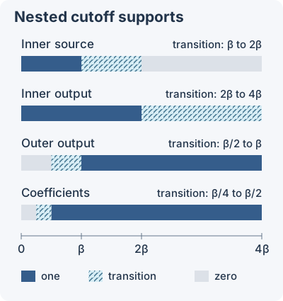
The inner output cutoff equals one on the inner input. The outer coefficients agree with the true compact coefficients wherever the outer output is nonzero. These support relations make the following cancellation exact.

Let $\mathcal{P}$ be the compact linearization. The localized inner correction obeys

$$\mathcal{P}{V}_i=f_i+R_{i}f+J_{i}f,$$

where the geometric mismatch $R_i$ is $O({\beta }^2)$, but the cutoff commutator $J_i$ is merely bounded. Define the outer source to be $f-f_i-J_{i}f$. Its correction then cancels the troublesome term. Only the geometric mismatch and an outer commutator remain. The latter has order at most three, so short-time interpolation gives

$$\Vert \mathcal{R}\Vert \le C({\beta }^2+{\eta }^{(1-\alpha )/4}).$$

For sufficiently small parameters, a Neumann series converts the approximate inverse into a bounded exact right inverse $D$. No injectivity assertion is needed.

Small corrected error, then a nonlinear fixed point

Let $E_c$ be the compact residual of $F$. A bounded inverse alone is insufficient: the proof needs $D{E}_c$ to be small. It splits the residual using the inner output cutoff so that the exterior part has exactly zero inner input.

Near the core, the weighted residual gains ${\beta }^{2-2\delta }$. For the exterior part, a higher Hölder exponent ${\alpha }^{\prime }>\alpha$ makes all four spatial derivatives small on the short interval. Denote by $X^{\prime }$ the norm retaining those spatial derivatives and their temporal Hölder seminorms, but omitting the first time derivative. Then

$$\begin{array}{rl}\Vert D{E}_c{\Vert }_{X^{\prime }}\le C(& {\beta }^{2-2\delta }+{\eta }^{({\alpha }^{\prime }-\alpha )/4}\\ & +{\eta }^{(1-\alpha )/4}).\end{array}$$

The time derivative cannot be made small by this reasoning: a zero-data solution has time derivative equal to its forcing at the initial face.

The nonlinear remainder $N(V)$ uses only spatial derivatives. On a small $X^{\prime }$ ball it is quadratic with a small Lipschitz constant. Thus

$$V=-D{E}_c-DN(V)$$

is a contraction. Its fixed point automatically belongs to the full parabolic space because $D$ maps the forcing space there; the equation recovers the omitted time derivative. The order of choices is fixed: first the uniform inverse constants, then the ball radius, then $\beta$, and finally $\eta$.

The bound on $v_{\ast }V$ preserves positivity of $1+v_{\ast }(F+V)$. Interior regularity supplies smoothness at every negative time, including both momentum endpoints through the auxiliary-sphere description. (OpenAI, 2026)

🏷️ Recover the singularity on projective space

At the fixed affine origin,

$$H(t,0)={\rho }^{-1}{G}^{\prime }(0)+O({\rho }^{-1+\delta }).$$

The exact scalar identity now gives the leading coefficient $a=-110G^{\prime }(0)>0$. Choose an interior slice, for instance $t=-T/2$, as the initial metric and translate time. The resulting smooth flow exists until elapsed time $T_{\ast }=T/2$ and has the announced $(T_{\ast }-t{)}^{-1/2}$ scalar divergence.

Smooth local uniqueness identifies this constructed trajectory with the unrestricted Calabi flow from that initial metric. Symmetry is used in the construction, not imposed on competing continuations. An extension beyond $T_{\ast }$ would have bounded scalar curvature on a compact smooth time neighborhood, contradicting the divergence. Biholomorphic pullback also preserves the maximum scalar-curvature magnitude and cannot remove this obstruction.

For a product with a stationary factor $(Y,\eta )$, scalar curvatures and their averages both add. The stationary contribution therefore cancels from $S-\bar{S}$, leaving exactly the original potential evolution. For $Y={\mathbb{CP}}^m$, scaling its Fubini–Study form by $(m+1)/11$ makes the two stationary reference factors have the same Einstein constant. This proves the claimed extension to every complex dimension $10+m$. (OpenAI, 2026)

The distinction from the Ricci-flow family is useful: this flow is fourth order in the potential, and the constructed singularity has explicitly unbounded scalar curvature. Here the certified profile, selected initial modes, and exact compact correction work together to exhibit one singular trajectory in a class that also contains a stationary metric.

🏷️ Key steps and proof outlines

The shooting problem matches exactly the two growing coordinates

The origin expansion has two free real parameters. At infinity the linear limiting equation has one stable real mode and two growing real modes. The half-line construction chooses a bounded tail after prescribing its stable coordinate; its growing coordinates are determined by integrals from infinity. Matching therefore requires two equations, exactly the number of origin parameters.

The certified finite shot is within $0.13R$ of the parameter vector in unstable coordinates, while the tail contribution is smaller than $0.25R$. The resulting correction map sends the parameter square into the strictly smaller square of radius $0.38R$. Brouwer supplies a fixed point, and ODE uniqueness joins the two solutions. The exact-arithmetic certificate controls these finite numerical inequalities. Positivity, differentiated tail expansions, and the compact PDE construction are additional analytic conclusions, not consequences of floating-point plots. (OpenAI, 2026)

A right inverse is enough because the initial data are selected

The flat similarity operator can have finitely many modes growing faster than the chosen weight. The two-sided discrete recurrence chooses those components using future forcing, while stable components use past forcing. This constructs one solution with the desired weighted bound; it does not prove all solutions with arbitrary initial data remain close to the profile.

That freedom is compatible with the theorem: the initial metric is chosen from the constructed singular trajectory. The inverse need only be a right inverse. Requiring zero initial data in the inner problem would remove the parameters used to control its finite unstable modes and would demand a different theorem.

The cutoff commutator is canceled before smallness is claimed

Let the localized inner inverse satisfy $\mathcal{P}{V}_i=f_i+R_{i}f+J_{i}f$. The geometric error $R_i$ is small, but the inner cutoff commutator $J_i$ need not be. Define the outer forcing as $f_o=f-f_i-J_{i}f$. The outer forward solution, multiplied by its output cutoff, satisfies $\mathcal{P}{V}_o=f_o+J_{o}f$. Adding gives the exact identity

$$\mathcal{P}(V_i+V_o)=f+(R_i+J_o)f.$$

Only the remaining outer commutator needs a small estimate. It contains at most three spatial derivatives because commuting a fourth-order operator with a cutoff lowers order by one. The zero-data outer solution has a small supremum norm on time scale $T\ll {\beta }^4$, and interpolation makes those lower derivatives small. Thus $\Vert R_i+J_o\Vert \le C[{\beta }^2+(T/{\beta }^4{)}^{(1-\alpha )/4}]$, allowing an exact Neumann-series correction. (OpenAI, 2026)

The nonlinear norm keeps precisely the derivatives used by the remainder

Short time does not make the first time derivative of a zero-data solution small at its initial face: there it equals the forcing. The contraction therefore uses a norm retaining four spatial derivatives and their temporal Hölder control, but omitting that time derivative. The nonlinear remainder depends only on the retained spatial data, so it is quadratic and Lipschitz there. The full right inverse and the equation recover the time derivative afterward.

The correction at the concentrating point is $O({\rho }^{-1+\delta })$, whereas the profile value is ${\rho }^{-1}{G}^{\prime }(0)$ with $G^{\prime }(0)<0$. Their ratio tends to zero. The scalar-curvature formula therefore retains the nonzero leading blowup coefficient, while positivity of the metric multiplier survives the small correction. This connects the weighted analytic estimates to a genuine finite-time geometric singularity.

🏷️ Manuscripts and verification scope

• A finite-time singularity of Calabi flow on projective space — pinned manuscript and companion source.

No family scope page was present at lean/docs/352.md in the pinned snapshot. This does not establish that all related formalization code is absent. No Lean build, axiom audit, or manuscript-to-formal-statement equivalence check was performed for these notes.

OpenAI collection provides prerequisites and the reading sequence; coverage register records completed and pending families.

🐻  OpenAI 2026. A finite-time singularity of Calabi flow on projective space.