Binary information and Hellinger contraction on the cube

Source and verification

This article explains family 119 of the October 6, 2026 OpenAI collection. Research conclusions are attributed to its manuscripts. The review covers statements, introductions, and selected proof mechanisms; it is not an independent verification of the complete proofs.

🏷️ A binary summary under product noise

Let $X$ be uniform on $\{-1,1{\}}^n$. Independently flip each coordinate with probability $\epsilon$, producing $Y$. The correlation is $\rho =1-2\epsilon$. A Boolean summary $f(X)\in \{-1,1\}$ retains some information about the full noisy vector $Y$.

The noise operator is

$$T_{\rho }u(y)=\mathbb{E}[u(X)\mid Y=y].$$

The uniform input makes the channel symmetric, so it can equivalently be defined by starting at $y$ and independently multiplying its coordinates by signs of mean $\rho$. Negative correlations are allowed. A coordinate function satisfies $T_{\rho }{x}_i=\rho x_i$.

A randomized binary summary $U$ is specified by its conditional mean $u(x)=\mathbb{E}[U\mid X=x]\in [-1,1]$. Such a function is called a soft binary channel. Noise is independent of $(X,U)$. The summary’s mean $m=\mathbb{E}u$ can be biased even though $X$ is uniform.

Use natural logarithms initially. Define binary entropy in mean coordinates by

$$\begin{array}{rl}h(r)& =-\frac{1+r}{2}\log \frac{1+r}{2}\\ & -\frac{1-r}{2}\log \frac{1-r}{2},\end{array}$$

with $0\log 0=0$, and put $L=\log 2$, $\psi (r)=L-h(r)$. The information carried by $u$ is

$$\begin{array}{rl}I(u)& =h(\mathbb{E}u)-\mathbb{E}h(u)\\ & =\mathbb{E}\psi (u)-\psi (\mathbb{E}u).\end{array}$$

This is $I(U;X)$, while $I(T_{\rho }u)=I(U;Y)$. The function $\psi$ is even and increases from zero to $L$ on $[0,1]$; its inverse below always means this nonnegative branch.

🏷️ Sharp information contraction

Soft-channel manuscript

For every finite dimension, every soft binary channel, and $-1\le \rho \le 1$,

$$I(T_{\rho }u)\le \psi (|\rho |{\psi }^{-1}(I(u))).$$

When $n\ge 1$, every soft coordinate $u(x)=a{x}_i$, $|a|\le 1$, attains equality. (OpenAI, 2026)

Indeed, a soft coordinate has mean zero, $I(u)=\psi (|a|)$, and noised information $\psi (|\rho a|)$. The theorem compares all channels at the same initial information with this explicit one-coordinate model. It does not hold the output mean fixed when asserting attainability.

For Boolean $f$, conditional entropy given $X$ is zero, so $I(f)=h(m)$. Set $r_m={\psi }^{-1}(h(m))$. The specialization gives

$$I(f(X);Y)\le \psi (|\rho |r_m)\le \psi (|\rho |).$$

At $m=0$, a signed coordinate attains the universal bound. When $0<|m|<1$ and $|\rho |>0$, the refined upper curve is strictly smaller, since $r_m<1$ and $\psi$ is strictly increasing. This does not assert that every prescribed biased Boolean mean has an optimizer attaining that curve.

Dividing by $L$ converts nats to bits. With binary entropy $h_2(p)=-p{\log }_{2}p-(1-p){\log }_2(1-p)$, the universal bound is

$$I_2(f(X);Y)\le 1-h_2(\epsilon ).$$

This is the Courtade–Kumar conclusion. Constant summaries have zero information. At $\rho =0$, the observation is independent of the summary; at $|\rho |=1$, it determines the input. The theorem includes these endpoints and the zero-dimensional constant case.

🏷️ A coordinate and two-bit parity

For the parity summary $f(x)=x_1{x}_2$, independence gives $T_{\rho }f={\rho }^2{x}_1{x}_2$. Both parity and a coordinate are balanced, so their retained information is respectively $\psi ({\rho }^2)$ and $\psi (\rho )$. For $0<\rho <1$, strict monotonicity of $\psi$ shows that parity retains less.

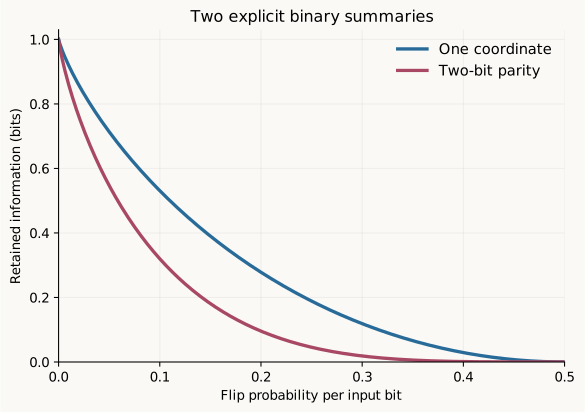
The curves plot the elementary formulas $1-h_2(\epsilon )$ and $1-h_2(2\epsilon (1-\epsilon ))$. Parity changes exactly when one of the two input bits flips. These analytic examples illustrate the comparison; they do not verify the theorem for arbitrary Boolean functions.

🏷️ Entropy production and effective amplitude

For an interior field $g:\{-1,1{\}}^n\to (-1,1)$, let

$$\begin{array}{c}N=\frac{1}{2}\sum _{i=1}^n(\mathrm{Id}-{\mathrm{flip}}_i),\\ P_t=T_{e^{-t}}=e^{-tN},\\ V(r)=\mathrm{atanh}r.\end{array}$$

Here ${\mathrm{flip}}_i$ changes only coordinate $i$. The semigroup preserves the mean. Since ${\psi }^{\prime }=V$, differentiation gives

$$\begin{array}{c}\frac{d}{dt}I(P_{t}g)=-D(P_{t}g),\\ D(g)=\mathbb{E}[V(g)Ng].\end{array}$$

Define the coordinate production profile $F$ by $F(\psi (r))=rV(r)$. If $D(g)\ge F(I(g))$, the effective amplitude $r_t={\psi }^{-1}(I(P_{t}g))$ obeys

$$V(r_t)r_t^{\prime }\le -r_{t}V(r_t).$$

For positive information, divide by $V(r_t)>0$ to obtain $r_t^{\prime }\le -r_t$. Thus $r_t\le e^{-t}{r}_0$, which gives the contraction curve. Zero information is treated separately; boundary-valued channels follow by approximation and continuity. The research difficulty is the production inequality, not this final differential comparison.

🏷️ Why the induction retains output bias

Split the cube into its two sections $g_{+},g_{-}$ along one coordinate. The production decomposes exactly as

$$\begin{array}{c}\begin{array}{rl}D(g)& =\frac{1}{2}(D(g_{+})+D(g_{-}))\\ & +\mathbb{E}c(g_{+},g_{-}),\end{array}\\ c(a,b)=\frac{1}{4}(a-b)(V(a)-V(b)).\end{array}$$

The last term is nonnegative because $V$ is increasing. An induction must make these joining edges pay the increase in the desired profile from the two sections to their parent. The source explains that the information-only profile $F$ does not satisfy the needed comparison for every coupled pair law. Ignoring the means too early loses the induction.

For $I<L$, put $S(I)=F(I)-2I$, and extend $S$ by zero for negative arguments. The manuscript introduces

$$\begin{array}{c}q=1-m^2,e=h(m)-I,\\ {\mathcal{B}}_m(I)=2I+qS(L-e/q),\end{array}$$

for $|m|<1$ and $0\le I<h(m)$. The stronger production claim is

$$D(g)\ge \max \{{\mathcal{B}}_m(I(g)),F(I(g))\}.$$

The factor $q$ is useful under splitting: sections of means $m\pm \delta$ have average variance factor $1-m^2-{\delta }^2$. Convexity can pool their surplus contributions with precisely that remaining capacity.

To prove the joining comparison, the source minimizes the joining cost over coupled pair laws with fixed section means and average conditional entropy. The optimizer has one interior pair and possibly the equal-output corners $(1,1)$ and $(-1,-1)$. A one-bit inequality pays for the interior pair. Adding a common output at a corner thins the interior mass, and a separate inequality shows that the required payment falls at least proportionally.

The maximum of the two profiles needs an additional argument. Above half information, ${\mathcal{B}}_m\ge F$; below it, the source controls the increment of the $F$ branch. For an optimizer using both corners, shifting the common mean until one corner disappears preserves the joining cost and increases the required increment in the relevant range. The one-corner comparison then pays the original state. These scalar and coupled-law estimates are the substantive interfaces supporting the dimension induction. (OpenAI, 2026)

🏷️ Hellinger affinity and a second contraction theorem

The companion uses a different concave profile,

$$Q(r)=\sqrt{1-r^2}.$$

For a nonconstant Boolean summary, let $P_{+}$ and $P_{-}$ be the conditional laws of $Y$ given $f(X)=1$ and $f(X)=-1$. Their Hellinger affinity is $A(P_{+},P_{-})={\sum }_y\sqrt{P_{+}(y)P_{-}(y)}$. Affinity one means the laws agree, while affinity zero means they have disjoint supports.

Writing $d=T_{\rho }f$, Bayes’ rule gives

$$\begin{array}{c}{P}_{\pm }(y)=2^{-n}\frac{1\pm d(y)}{1\pm m},\\ A(P_{+},P_{-})=\frac{\mathbb{E}Q(d)}{Q(m)}.\end{array}$$

Hellinger manuscript

For every Boolean function on a positive-dimensional uniform cube, with arbitrary output mean $m$, and every $\rho \in [-1,1]$,

$$Q(m)-\mathbb{E}Q(T_{\rho }f)\le 1-Q(\rho ).$$

Signed coordinates attain equality. (OpenAI, 2026a)

For nonconstant functions, the left side is the weighted affinity loss $Q(m)(1-A)$. Constant functions satisfy the inequality directly; the conditional-law formula is not used when a conditioning event has probability zero. Arbitrary output bias does not change the uniform input assumption.

🏷️ Deriving the information bound from affinity

The implication to Courtade–Kumar can be written out using one scalar function:

$$\begin{array}{c}\phi (t)=h_2\left(\frac{1-\sqrt{1-t^2}}{2}\right),\\ 0\le t\le 1.\end{array}$$

It is increasing and convex. For example, with $v=\sqrt{1-t^2}$, the sign of ${\phi }^{\prime \prime }$ is the sign of $\log ((1+v)/(1-v))-2v$, which is nonnegative because it vanishes at zero and has derivative $2v^2/(1-v^2)\ge 0$.

Set $h=Q(m)$, $b=\mathbb{E}Q(d)$, and $s=Q(\rho )$. The identity $h_2((1+u)/2)=\phi (Q(u))$ and Jensen’s inequality yield

$$I_2(f(X);Y)\le \phi (h)-\phi (b).$$

Concavity of $Q$ gives $b\le h$. The Hellinger theorem bounds $\delta =h-b$ by $1-s$. For a convex function, an increment of fixed length grows when its interval moves to the right. Since $h\le 1$,

$$\begin{array}{rl}\phi (h)-\phi (b)& \le \phi (1)-\phi (1-\delta )\\ & \le \phi (1)-\phi (s)\\ & =1-h_2(\epsilon ).\end{array}$$

This proves the universal Boolean information consequence from the companion’s inequality. It does not establish the stronger soft-channel theorem or its mean-dependent production estimate.

🏷️ The companion’s induction and continuation

Write $s=\sqrt{1-{\rho }^2}$. For $s\le 0.84$, the source compresses to increasing Boolean functions and uses an asymmetric dimension induction. A concave profile $G$ satisfies $G(p)+G(1-p)=2Q(2p-1)$. Averaging the bounds for $f$ and its reflected increasing counterpart recovers the desired symmetric profile. A sheared two-section comparison controls the mixing gain before substituting induction hypotheses.

For $s\ge 0.84$, an assumed first failure would force the semigroup energy to be no larger than the coordinate energy. A transformed field with derivative $Q^{-3/2}$ supplies a Dirichlet-energy lower bound. Near zero bias, a calibrated symmetric comparison retains the exact coordinate cost; intermediate biases use even–odd Fourier decomposition; large biases use forward and reverse cube norm estimates. Together the estimates exclude the crossing except for signed coordinates, where equality is already known.

This proof uses fixed exact-arithmetic certificates for scalar inequalities. Their domains and sizes are independent of the cube dimension, and the displayed decimal thresholds denote exact rationals. No certificate program was executed for this article. The source review therefore explains the proof dependencies without independently certifying those finite calculations.

🏷️ Key steps and proof outlines

An exact reserve for joining two sections

The production argument’s essential scalar object is the perspective

$$R(v,e)=vS(L-e/v),$$

where $S=F-2I$ is extended by zero below zero. Think of $v$ as an available variance capacity and $e$ as the remaining conditional entropy. This is an interpretation of a numerical profile; it does not assert that a channel literally splits into independent components. (OpenAI, 2026b)

For section means $a=m+\delta$ and $b=m-\delta$, put $\alpha =1-m^2$ and $\beta =\alpha -{\delta }^2$. Their average variance capacity is exactly $\beta$, whereas the parent capacity is $\alpha$. If $e$ is the average section entropy and $J=h(m)-(h(a)+h(b))/2$ the information gained from the joining bit, convexity of the perspective pools the child reserves. The extra payment required at the join is at most

$$W(m,\delta ,e)=2J+R(\alpha ,e)-R(\beta ,e).$$

This formula isolates what the joining edges must pay. The linear part costs $2J$; the remaining difference measures the capacity gained when the section means merge.

Common-output mixing preserves the payment inequality

The canonical coupled law has one interior pair and possibly equal-output atoms at $(1,1)$ and $(-1,-1)$. The corners contribute no joining cost because their two outputs agree. If an interior law is retained with probability $\tau$ and the positive common output is added otherwise, its parameters become

$$(m,\delta ,e)⟼(1-\tau +\tau m,\tau \delta ,\tau e).$$

The source proves $W$ at the new parameters is at most $\tau W$ at the old ones. Its proof fixes the ratios $\delta /(1-m)$ and $e/(1-m)$ and differentiates along that ray. A curvature bound for $S$ and a logarithmic comparison for $\alpha /\beta$ show that $W/(1-m)$ is nondecreasing. Moving to the smaller value $\tau (1-m)$ yields the required inequality. Reflection gives the negative common-output case.

Starting from the interior pair, add the two corners successively. The two retention factors multiply to the interior mass. Since the one-bit inequality pays the interior pair’s $W$, the total joining cost pays the entire mixed law. Coupled-law minimization then transfers this bound to arbitrary section pairs. This is why retaining the mean makes induction possible: the variance capacity tracks precisely the change caused by adding common outputs.

From local joining to the noise curve

The cube decomposition sums productions inside the sections and across the joining coordinate. Induction applies the child profiles, and the local joining inequality pays their deficit relative to the parent. The separate upgrade argument supplies the maximum with the unbiased profile $F(I)$. Consequently, along $g_t=T_{e^{-t}}g$,

$$-I^{\prime }(t)\ge F(I(t))=r_t\mathrm{atanh}(r_t),I(t)=\psi (r_t).$$

At positive information, differentiating $I(t)$ and cancelling the positive factor $\mathrm{atanh}(r_t)$ gives $(e^t{r}_t{)}^{\prime }\le 0$. Integrating proves the claimed contraction. Interior approximation handles values $\pm 1$, where the entropy derivative is infinite, and continuity restores the boundary channels.

The Hellinger companion uses a different local profile and then a continuation argument. At a hypothetical first crossing, the deficit’s derivative must point toward failure; the semigroup energy estimates rule out that direction in their respective bias ranges. Exact scalar certificates support those estimates. The subsequent Jensen argument converts its affinity loss into the universal Boolean information bound, but does not replace the stronger reserve argument for soft channels. (OpenAI, 2026a)

See Also

• Fourier degree and sensitivity introduces another use of cube functions and spectral decompositions, with different extremal quantities.
• Circuit lower bounds uses random restrictions and correlation estimates; noise contraction here is a functional inequality on the full uniform cube.

🏷️ Manuscripts and verification scope

• Sharp binary-information contraction on the discrete cube — pinned manuscript and companion source.
• Hellinger contraction with arbitrary Boolean output bias — pinned manuscript and companion source.

The family scope page describes selected formalization coverage. The scope selects the soft-channel contraction, the Boolean information consequence, and a mean-dependent production inequality. It does not list the separate Hellinger manuscript as a formalized headline theorem. No Lean build, axiom audit, or manuscript-to-formal-statement equivalence check was performed for these notes.

OpenAI collection provides prerequisites and the reading sequence; coverage register records completed and pending families.

🐻  OpenAI 2026a. Hellinger contraction with arbitrary Boolean output bias.

🐻  OpenAI 2026b. Sharp binary-information contraction on the discrete cube.