on the KLS conjecture through cumulants and polynomial bounds

Overview

A log-concave probability distribution has no separated islands of mass, but it can have complicated geometry in high dimension. The Kannan–Lovász–Simonovits conjecture asks whether its largest linear fluctuation already determines its Poincaré constant, up to a universal factor.

Two October 2026 preprints establish a dimension-free bound. Song and Zhang develop a method that converts bounds for specially centered polynomials into a spectral gap, and then repeatedly improves those bounds. Bizeul, Klartag, and Lehec use the Song–Zhang criterion with a different input: estimates for cumulants of every order, followed by a convex construction in a larger dimension. This exposition develops the shared preliminaries, the cumulant and suspension argument, and the quantitative mechanisms that close the polynomial iteration.

🏷️ Log-concave measures and the KLS constant

A full-dimensional probability measure on ${\mathbb{R}}^n$ is log-concave if it has density

$$d\mu (x)=e^{-V(x)}dx$$

for a convex function $V:{\mathbb{R}}^n\to \mathbb{R}\cup \{+\infty \}$. The additive constant in $V$ normalizes the integral. Allowing $V=+\infty$ includes uniform probability measures on convex bodies. Gaussian distributions and products of exponential distributions are other examples.

For $X\sim \mu$, write

$$\begin{array}{rl}m& =\mathbb{E}X,\\ \Sigma & =\mathbb{E}[(X-m)(X-m{)}^{\mathsf{T}}].\end{array}$$

The measure is isotropic if $m=0$ and $\Sigma =I_n$. When $\Sigma$ is positive definite, the affine transformation

$$Y={\Sigma }^{-1/2}(X-m)$$

makes the law isotropic. Affine images preserve log-concavity. Isotropy fixes the scale in every direction; it does not imply rotational symmetry or independence of the coordinates.

The Poincaré constant $C_P(\mu )$ is the smallest constant such that

$${\mathrm{Var}}_{\mu }(f)\le C_P(\mu )\int |\nabla f{|}^{2}d\mu .$$

Initially one can take smooth functions with finite variance and energy. The resulting inequality extends to locally Lipschitz functions by approximation. A function with large variance and small gradient energy is a slowly varying obstruction to concentration; the Poincaré constant measures the worst such obstruction.

For a linear function $f(x)=⟨u,x⟩$,

$$\begin{array}{rl}{\mathrm{Var}}_{\mu }(f)& =u^{\mathsf{T}}\Sigma u,\\ \int |\nabla f{|}^{2}d\mu & =|u{|}^2.\end{array}$$

Consequently,

$$C_P(\mu )\ge \Vert \Sigma {\Vert }_{\mathrm{op}}.$$

KLS asks for a matching upper bound, with one constant for every dimension and every log-concave measure. In isotropic position, it asks whether the variance of an arbitrary function can exceed its gradient energy by more than a universal factor.

Boundary expansion and the reciprocal convention

For a measurable set $A$, define its outer boundary measure by

$$\begin{array}{rl}& {\mu }^{+}(A)\\ & =\underset{\epsilon \downarrow 0}{\mathrm{liminf}}\frac{\mu (A+\epsilon B_2^n)-\mu (A)}{\epsilon }.\end{array}$$

Here $B_2^n$ is the Euclidean unit ball. The Cheeger constant and its reciprocal are

$$\begin{array}{rl}& h(\mu )\\ & =\underset{0<\mu (A)<1}{\inf }\frac{{\mu }^{+}(A)}{\min \{\mu (A),1-\mu (A)\}},\\ & \psi (\mu )=h(\mu {)}^{-1}.\end{array}$$

A small Cheeger constant means that some set separates substantial masses with little boundary. Cheeger’s inequality and its reverse for log-concave measures give

$$C_P(\mu )\asymp \psi (\mu {)}^2.$$

Thus the quantity

$${\psi }_n=\underset{\begin{array}{c}\mu \text{ isotropic}\\ \mu \text{ log-concave on }{\mathbb{R}}^n\end{array}}{\sup }\psi (\mu )$$

is bounded universally exactly when the isotropic Poincaré constants are. This convention agrees with Song–Zhang and with on a sharp quadratic-form inequality and the KLS constant, which supplies a principal input below. A bound for $C_P$ becomes a square-root bound for ${\psi }_n$.

The geometric content is already visible for a convex body: half-space cuts are governed by one-dimensional marginals, and their scale is controlled by directional variance. KLS says that complicated cuts cannot have a much worse expansion scale.

🏷️ The two papers and their theorem

Dimension-free KLS bound

There is a universal $C<\infty$ such that every isotropic log-concave probability measure $\mu$ on ${\mathbb{R}}^n$ satisfies

$$C_P(\mu )\le C.$$

Equivalently, for an arbitrary full-dimensional log-concave measure,

$$\Vert \Sigma {\Vert }_{\mathrm{op}}\le C_P(\mu )\le C\Vert \Sigma {\Vert }_{\mathrm{op}}.$$

These are Theorem 1.1 of Bizeul–Klartag–Lehec and Theorem 9.1 of Song–Zhang, in the versions specified below (Bizeul, Klartag & Lehec, 2026; Song & Zhang, 2026).

For the upper affine bound, apply the isotropic theorem to $g(y)=f(m+{\Sigma }^{1/2}y)$. The chain rule gives

$$\begin{array}{rl}|\nabla g(y){|}^2& =⟨\Sigma \nabla f,\nabla f⟩\\ & \le \Vert \Sigma {\Vert }_{\mathrm{op}}|\nabla f{|}^2.\end{array}$$

If the support lies in a proper affine subspace, the corresponding statement is interpreted within that subspace, with the intrinsic gradient. A point mass has zero variance and causes no difficulty.

Version dependence

The source versions matter because the second paper changed its conclusion between submissions.

Paper and version	Date	Conclusion
Song–Zhang, v1	October 1, 2026	${\psi }_n\lesssim 4^{{\log }^{\ast }(n+2)}$
Bizeul–Klartag–Lehec, v1	October 4, 2026	$C_P\lesssim 1$, using the Song–Zhang criterion
Song–Zhang, v2	October 4, 2026	$C_P\lesssim 1$ and ${\psi }_n\lesssim 1$

Here ${\log }^{\ast }x$ counts the successive natural logarithms needed to bring $x$ to at most one. The earlier Song–Zhang estimate corresponds to $C_P\lesssim 16^{{\log }^{\ast }(n+2)}$ (Song & Zhang, 2026b). It explains the historical comparison in the introduction of Bizeul–Klartag–Lehec. The discussion below uses Bizeul–Klartag–Lehec v1 and Song–Zhang v2, including the latter’s final bounded-cost argument.

🏷️ Exponential tilts, cumulants, and centered polynomials

The logarithmic Laplace transform of $\mu$ is

$${\Lambda }_{\mu }(z)=\log \int e^{⟨z,x⟩}d\mu (x).$$

For a full-dimensional log-concave probability measure, this is finite in a neighborhood of zero. The exponential tilt in direction $z$ is

$$d{\mu }_z(x)=e^{⟨z,x⟩-{\Lambda }_{\mu }(z)}d\mu (x).$$

Tilting changes the potential by a linear function, so it preserves convexity. For an observable $f$, define its tilt average

$$F_f(z)=\int fd{\mu }_z.$$

Differentiating the quotient defining this expectation gives

$${\partial }_{z_i}{F}_f(z)={\mathrm{Cov}}_{{\mu }_z}(f,X_i).$$

At $z=0$, isotropy therefore controls the first derivative:

$$\begin{array}{c}\nabla F_f(0)=\mathbb{E}[Xf(X)],\\ |\nabla F_f(0)|\le \Vert f{\Vert }_{L^2(\mu )}.\end{array}$$

The inequality follows by testing against a unit vector $u$ and using Cauchy–Schwarz with $\mathbb{E}⟨u,X{⟩}^2=1$. Higher derivatives encode increasingly complicated correlations. Both proofs seek control of the whole derivative tensor, with a constant that grows at most exponentially in its order after the Taylor factorial is removed.

Tensor norms and cumulants

For an order-$d$ tensor $T$, use the Hilbert–Schmidt norm

$$|T{|}^2=\sum _{i_1,\dots ,i_d=1}^n{T}_{i_1\cdots i_d}^2.$$

The sum is over all ordered indices. For matrices this is the usual Frobenius norm. It is generally much stronger to control this norm than to bound a multilinear form separately on unit vectors.

The cumulant tensor of order $m$ is

$${\kappa }_m^{\mu }={\nabla }^m{\Lambda }_{\mu }(0).$$

The first two cumulants are the mean and covariance. For a centered vector, the third is its third moment tensor. The fourth subtracts all covariance pairings:

$$\begin{array}{rl}({\kappa }_4{)}_{ijkl}=& \mathbb{E}[X_i{X}_j{X}_k{X}_l]\\ & -{\Sigma }_{ij}{\Sigma }_{kl}-{\Sigma }_{ik}{\Sigma }_{jl}\\ & -{\Sigma }_{il}{\Sigma }_{jk}.\end{array}$$

Taking a logarithm removes the products contributed by independent groups of variables. This explains why cumulants are the natural quantities in the stochastic recursion later on.

For $u\in {\mathbb{R}}^n$, write ${\kappa }_m(u)={\kappa }_m(u,\cdot ,\dots ,\cdot )$. Bizeul–Klartag–Lehec estimate this $(m-1)$-tensor:

$$|{\kappa }_m(u){|}^2\le K^{m-1}((m-1)!{)}^2|u{|}^2.$$

Only one slot is fixed. The remaining slots are all summed in Hilbert–Schmidt norm. This is a dimension-free bound on the linear map from $u$ to the entire tensor slice.

Independent centered exponential coordinates

Let $X_i=Y_i-1$, where the $Y_i$ are independent exponential variables of mean one. Since

$$\log \mathbb{E}{e}^{z{X}_i}=-z-\log (1-z),$$

their cumulants satisfy ${\kappa }_m(X_i)=(m-1)!$ for $m\ge 2$. Independence gives

$${\kappa }_m=(m-1)!\sum _{i=1}^n{e}_i^{\otimes m}.$$

Thus

$$\begin{array}{rl}|{\kappa }_m(u){|}^2& =((m-1)!{)}^2|u{|}^2,\\ |{\kappa }_m{|}^2& =n((m-1)!{)}^2.\end{array}$$

The factorial growth is necessary. The full tensor norm also necessarily sees dimension; the one-slot estimate has the appropriate normalization.

Appell polynomials and the dual formulation

Define symmetric tensor-valued Appell polynomials ${\mathcal{A}}_d^{\mu }(x)$ by the generating identity

$$e^{⟨z,x⟩-{\Lambda }_{\mu }(z)}=\sum _{d\ge 0}\frac{1}{d!}⟨{\mathcal{A}}_d^{\mu }(x),z^{\otimes d}⟩.$$

At any specified degree this is an identity of formal Taylor coefficients. It requires only finitely many moments. For an isotropic measure,

$$\begin{array}{rl}{\mathcal{A}}_1(x)& =x,\\ {\mathcal{A}}_2(x)& =x^{\otimes 2}-I,\\ ({\mathcal{A}}_3(x){)}_{ijk}& =x_i{x}_j{x}_k-{\delta }_{ij}{x}_k\\ & -{\delta }_{ik}{x}_j-{\delta }_{jk}{x}_i\\ & -\mathbb{E}[X_i{X}_j{X}_k].\end{array}$$

For a symmetric coefficient tensor $T$, set

$$P_d^{\mu }[T](x)=⟨T,{\mathcal{A}}_d^{\mu }(x)⟩.$$

It is the unique polynomial with leading term $⟨T,x^{\otimes d}⟩$ satisfying

$$\begin{array}{c}\mathbb{E}[D^j{P}_d^{\mu }[T]]=0(0\le j<d),\\ D^d{P}_d^{\mu }[T]=d!T.\end{array}$$

These conditions remove the means of all lower derivatives, rather than merely removing the mean of the polynomial. For example, subtracting a constant from a cubic does not center its first derivative.

Define

$$\begin{array}{rl}{K}_d(\mu )& =\underset{|T|=1}{\sup }{\mathrm{Var}}_{\mu }(P_d^{\mu }[T]),\\ c_d(\mu )& =\frac{\sqrt{K_d(\mu )}}{d!},\\ {\mathcal{T}}_{d}f& =\frac{1}{d!}{\nabla }^d{F}_f(0).\end{array}$$

The supremum in $K_d$ is over symmetric tensors. Differentiation under the integral gives the exact pairing

$$⟨{\mathcal{T}}_{d}f,T⟩=\frac{1}{d!}\mathbb{E}[f{P}_d^{\mu }[T]].$$

Taking the two operator norms shows

$$\Vert {\mathcal{T}}_d:L^2(\mu )\to {\mathrm{Sym}}^d({\mathbb{R}}^n)\Vert =c_d(\mu ).$$

This identity connects the papers: a tilt-derivative estimate and an Appell variance estimate are dual descriptions of the same bound.

Every polynomial $q$ of degree at most $s$ also has the exact expansion

$$q-\mathbb{E}q=\sum _{k=1}^s\frac{1}{k!}{P}_k^{\mu }[\mathbb{E}{D}^{k}q].$$

Indeed, the two sides have the same expected derivatives of each order and the same mean; descending from the leading coefficient proves equality. The triangle inequality yields

$$\sqrt{{\mathrm{Var}}_{\mu }(q)}\le \sum _{k=1}^s{c}_k(\mu )|\mathbb{E}{D}^{k}q|.$$

Appell polynomials for a general measure need not be orthogonal. The last estimate is an $L^2$ triangle inequality, not a Parseval identity (Song & Zhang, 2026a, sec.2.3).

An exact one-dimensional example

For $X=Y-1$ with $Y$ exponential of mean one, the generating function is $(1-z)e^{z(x+1)}$. Hence, for $d\ge 1$,

$$P_d(x)=(x+1{)}^d-d(x+1{)}^{d-1}.$$

Using $\mathbb{E}{Y}^k=k!$ gives

$$\begin{array}{rl}\mathbb{E}{P}_d(X)& =0,\\ \mathbb{E}{P}_d(X{)}^2& =d^2(2d-2)!,\\ c_d^2& =\left(\genfrac{}{}{0ex}{}{2d-2}{d-1}\right).\end{array}$$

Thus $c_d$ has exponential growth, up to a polynomial factor. By comparison, for the standard Gaussian the Appell polynomials are the probabilists’ Hermite polynomials, whose squared norm is $d!$, so $c_d=1/\sqrt{d!}$. These examples explain why a universal exponentially growing bound is a natural target.

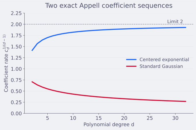
The coefficient rate $c_d^{1/(d-1)}$ for these exact one-dimensional formulas. The exponential example approaches $2$. The plot illustrates normalization; it supplies no evidence about arbitrary log-concave measures.

🏷️ Analytic preliminaries and the common criterion

A convenient preliminary reduction is to regular measures: $V$ is smooth, its derivatives have at most polynomial growth, and

$$aI⪯D^{2}V(x)⪯bI$$

for some $a,b>0$. These constants can depend on the measure. Convolution with a small Gaussian, followed by multiplication by $e^{-\delta |x{|}^2/2}$ and normalization, produces such approximations. Recentring and whitening restore isotropy. The approximations converge weakly with their fixed-order moments.

The associated diffusion generator is

$$L=\Delta -⟨\nabla V,\nabla ⟩,H=-L.$$

Integration by parts gives

$$\int uHvd\mu =\int ⟨\nabla u,\nabla v⟩d\mu .$$

Thus $H$ is nonnegative and self-adjoint in $L^2(\mu )$ after taking its natural closure. Constants form its kernel. On mean-zero functions it has a positive first eigenvalue

$$\lambda =C_P(\mu {)}^{-1}.$$

Regularity supplies a normalized first eigenfunction $f$ with $Hf=\lambda f$, $\mathbb{E}f=0$, and $\Vert f{\Vert }_2=1$. The inverse $H^{-1}$ and inverse square root $H^{-1/2}$ are defined on the mean-zero subspace by spectral calculus. In particular,

$$\begin{array}{rl}\Vert \nabla H^{-1}g{\Vert }_2^2& =⟨g,H^{-1}g⟩\\ & \le {\lambda }^{-1}\Vert g{\Vert }_2^2.\end{array}$$

The crucial curvature identity is the integrated Bochner formula:

$$\begin{array}{rl}& \Vert Lu{\Vert }_2^2=\Vert D^{2}u{\Vert }_2^2\\ & +\int ⟨D^{2}V\nabla u,\nabla u⟩d\mu .\end{array}$$

Convexity makes the last term nonnegative; regularity bounds it below by $a\Vert \nabla u{\Vert }_2^2$. All tensor-valued identities below mean the sum of the corresponding scalar identities over components. The domain and approximation details are treated in Bizeul–Klartag–Lehec, Section 2, and Song–Zhang, Section 3.

Song–Zhang tilt-derivative criterion

Let $\mu$ be centered and regular, with covariance at most $I$. If $R\ge 1$ satisfies

$$|{\mathcal{T}}_{d}f|\le R^d\Vert f{\Vert }_2$$

for every $d\ge 1$ and every $f\in L^2(\mu )$, then

$$C_P(\mu )\le C{R}^2.$$

This is the form proved in Bizeul–Klartag–Lehec, Theorem 3.1, from Song–Zhang’s polynomial-to-curvature method (Bizeul, Klartag & Lehec, 2026; Song & Zhang, 2026a).

The conclusion is uniform in the auxiliary curvature $a$. Sending $a$ to zero in the regular approximation therefore recovers measures with flat potentials or bounded support.

flowchart TD
    Q["Quadratic<br/>variance bound"] --> C["Cumulant bounds<br/>at all orders"]
    C --> S["Convex<br/>suspension"]
    S --> T["Tilt derivative<br/>bounds"]
    Q --> P["Appell variance<br/>bounds"]
    P --> R["Curvature<br/>refinement"]
    R --> T
    T --> G["Universal<br/>spectral gap"]

The left branch is the cumulant construction. The right branch improves the polynomial bounds until their coefficient radius is universal. The two branches share the quadratic input and the analytic passage from coefficients to a spectral gap.

🏷️ Proof of the tilt-derivative criterion

The proof assumes that $\lambda$ is very small and constructs a sequence whose energy must eventually disappear. Every possible mechanism for that disappearance is then bounded by a quantity too small to account for the loss.

Centered inverse-gradient iteration

Write ${\nabla }_{0}u=\nabla u-\mathbb{E}\nabla u$. Starting with $h_1=f$, set

$$\begin{array}{rl}{h}_{i+1}& ={\alpha }_{i+1}{H}^{-1}{\nabla }_0{h}_i,\\ {\alpha }_{i+1}& =\frac{\Vert {\nabla }_0{h}_i{\Vert }_2}{\Vert \nabla H^{-1}{\nabla }_0{h}_i{\Vert }_2}.\end{array}$$

If the centered gradient vanishes, set all subsequent iterates to zero. Each iteration adds a tensor index. The normalization gives the exact identity

$$\Vert \nabla h_{i+1}{\Vert }_2^2=\Vert {\nabla }_0{h}_i{\Vert }_2^2.$$

Define energy and centering loss by

$$v_i=\Vert \nabla h_i{\Vert }_2^2,p_i=|\mathbb{E}\nabla h_i{|}^2.$$

Then $v_1=\lambda$ and

$$\begin{array}{c}{v}_{i+1}=v_i-p_i,\\ \lambda =v_{N+1}+\sum _{i=1}^N{p}_i.\end{array}$$

The normalization also implies ${\alpha }_{i+1}^2\ge \lambda$ whenever the iterate is nonzero.

The new tensor need not be symmetric. Measure this difficulty through the exact squared defect

$${\chi }_i=\Vert D^2{h}_i-{\alpha }_{i+1}\nabla h_{i+1}{\Vert }_2^2.$$

Integration by parts shows that the two terms have the projection identity

$$⟨D^2{h}_i,\nabla h_{i+1}{⟩}_{L^2}={\alpha }_{i+1}{v}_{i+1}.$$

Consequently,

$$\Vert D^2{h}_i{\Vert }_2^2=\Vert L{h}_{i+1}{\Vert }_2^2+{\chi }_i.$$

Combining this with Bochner gives

$$\Vert L{h}_i{\Vert }_2^2\ge \Vert L{h}_{i+1}{\Vert }_2^2+{\chi }_i+a{v}_i.$$

Since $\Vert L{h}_1{\Vert }_2^2={\lambda }^2$, summation proves

$$\sum _{i\ge 1}{\chi }_i\le {\lambda }^2,a\sum _{i\ge 1}{v}_i\le {\lambda }^2.$$

In particular $v_i\to 0$. Let $N$ be the first index with $v_{N+1}<\lambda /2$. Up to that stopping index,

$$\begin{array}{c}\sum _{i=1}^N{p}_i>\lambda /2,\\ \lambda \le {\alpha }_i^2\le 2\lambda (2\le i\le N).\end{array}$$

The upper bound follows from ${\alpha }_i^2{v}_i=\Vert L{h}_i{\Vert }_2^2\le {\lambda }^2$ and $v_i\ge \lambda /2$.

Taylor identities and partial symmetry

The generator of the tilted measure is $L_z=L+z\cdot \nabla$. Integrating $L_{z}u$ against its invariant measure yields

$$F_{-Lu}(z)=⟨z,F_{\nabla u}(z)⟩.$$

Let ${\mathcal{S}}_q$ average a tensor over permutations of its first $q$ slots. Taking Taylor coefficients gives

$$\begin{array}{rl}{\mathcal{T}}_1(-Lu)& =\mathbb{E}\nabla u,\\ {\mathcal{T}}_{d+1}(-Lu)& ={\mathcal{S}}_{d+1}{\mathcal{T}}_d(\nabla u).\end{array}$$

The factorial normalization is essential: exactly one derivative hits the explicit factor $z$, and the resulting $d+1$ choices cancel the ratio $(d+1)!/d!$.

A partial symmetrization can annihilate an arbitrary tensor. The iterates have enough approximate symmetry to avoid that obstruction. Their adjacent-slot errors are controlled by ${\chi }_i$, since $D^2{h}_i$ is symmetric in its two derivative slots. Propagating those errors with ${\alpha }_i{\nabla }_0{H}^{-1}$ costs at most $\sqrt{2}$ per iteration before $N$.

The algebraic recovery statement used here is:

Recovery from two symmetric blocks

Suppose $T$ has at least $3d$ slots, is symmetric in its first $d$ slots, and is separately symmetric in the next $2d$ slots. Then

$$|T|\le \left(\genfrac{}{}{0ex}{}{2d}{d}\right)|{\mathcal{S}}_{2d}T|\le 4^d|{\mathcal{S}}_{2d}T|.$$

The extra block matters: symmetrizing just two equally sized blocks all the way to a fully symmetric tensor would not have such an injectivity statement.

Proof of the block recovery estimate

Put $\Omega =\{1,\dots ,3d\}$. For each $d$-element subset $F$, let $T_F$ be the tensor with its first symmetric block moved into $F$. Double counting gives

$$\begin{array}{rl}& \sum _{|E|=2d}{\left|\sum _{\begin{array}{c}F\subset E\\ |F|=d\end{array}}{T}_F\right|}^2\\ & =\sum _{s=0}^d\left(\genfrac{}{}{0ex}{}{d}{s}\right)\sum _{|S|=s}{\left|\sum _{\begin{array}{c}F\supset S\\ |F|=d\end{array}}{T}_F\right|}^2.\end{array}$$

To check the equality, expand both squared norms. If $|F\cap F^{\prime }|=r$, the coefficient of $⟨T_F,T_{F^{\prime }}⟩$ on either side is $\left(\genfrac{}{}{0ex}{}{d+r}{d}\right)$, by Vandermonde’s identity. Keeping the nonnegative term $s=d$ bounds the right side below by $\left(\genfrac{}{}{0ex}{}{3d}{d}\right)|T{|}^2$. Each inner sum on the left is a permuted copy of $\left(\genfrac{}{}{0ex}{}{2d}{d}\right){\mathcal{S}}_{2d}T$, and $\left(\genfrac{}{}{0ex}{}{3d}{2d}\right)=\left(\genfrac{}{}{0ex}{}{3d}{d}\right)$. Cancelling gives the claim (Bizeul, Klartag & Lehec, 2026, p.L emma 2.2).

Combining recovery, the adjacent-slot estimates, and the Taylor identity yields the degree-doubling estimate

$$\begin{array}{rl}& |{\mathcal{T}}_d({\nabla }_0{h}_i){|}^2\\ & \le (C\lambda {)}^d|{\mathcal{T}}_{2d}({\nabla }_0{h}_{i-d}){|}^2\\ & +\frac{C^d{R}^{2d}}{\lambda }\sum _{j=i-2d+1}^{i-1}{\chi }_j.\end{array}$$

valid for $2d\le i\le N$. The first term transports the Taylor degree from $d$ to $2d$; the second charges the failure of symmetry to the finite Bochner defect budget (Bizeul, Klartag & Lehec, 2026, p.L emmas 3.2–3.8).

The finite dyadic contradiction

Set

$$S_d=\sum _{i=1}^{N-d}|{\mathcal{T}}_d({\nabla }_0{h}_i){|}^2,$$

with an empty sum interpreted as zero. The terms with $i<2d$ are bounded directly by $\lambda R^{2d}$. In the remaining terms, each ${\chi }_j$ appears at most $2d$ times. Therefore

$$S_d\le (C\lambda {)}^d{S}_{2d}+4d{C}^d\lambda R^{2d}.$$

Suppose $\lambda R^2\le (100C^2{)}^{-1}$. Multiplication by $(C\lambda {)}^{d-1}$ gives

$$(C\lambda {)}^{d-1}{S}_d\le (C\lambda {)}^{2d-1}{S}_{2d}+\frac{4d}{100^d}.$$

Sum at $d=1,2,4,\dots$ until the first $d\ge N$, when $S_d=0$. The intermediate terms telescope, so

$$S_1\le 4\sum _{d=1}^{\infty }\frac{d}{100^d}<\frac{1}{20}.$$

Finally, integration by parts against coordinate functions gives $p_1\le {\lambda }^2$, while for $i\ge 2$,

$$p_i={\alpha }_i^2|{\mathcal{T}}_1({\nabla }_0{h}_{i-1}){|}^2.$$

Hence

$$\sum _{i=1}^N{p}_i\le {\lambda }^2+2\lambda S_1<\lambda /2,$$

contradicting the definition of $N$. Thus $\lambda \gtrsim R^{-2}$. The argument used a finite stopping index and a finite sequence of doubled degrees; neither needs a uniform bound before the contradiction.

🏷️ The quadratic input and stochastic localization

The starting estimate for both approaches is the sharp quadratic-form inequality

$$\mathrm{Var}(X^{\mathsf{T}}MX)\le 8\mathrm{Tr}(M^2)$$

for isotropic log-concave $X$ and every symmetric $M$ (Letwin, 2026). Its moment-map proof is developed in on a sharp quadratic-form inequality and the KLS constant. This is a substantive geometric input; isotropy alone does not imply it.

For a vector $u$, Cauchy–Schwarz gives

$$\begin{array}{rl}& |⟨{\kappa }_3(u),M⟩{|}^2\\ & =|\mathrm{Cov}(⟨u,X⟩,X^{\mathsf{T}}MX){|}^2\\ & \le 8|u{|}^2|M{|}^2.\end{array}$$

Taking the supremum over symmetric $M$ of Hilbert–Schmidt norm one proves

$$|{\kappa }_3(u){|}^2\le 8|u{|}^2.$$

The next task is to propagate this estimate to all orders. Stochastic localization supplies a process in which the next cumulant appears as the noise coefficient of the current one.

Localization with inverse covariance

Begin with a compactly supported isotropic log-concave measure. This reduction keeps the moment calculations bounded; the final fixed-order estimates pass to general measures by truncation and whitening.

Let $B_t$ be standard Brownian motion. Define random tilted measures by

$$d{\mu }_t(x)=Z_t^{-1}{e}^{⟨c_t,x⟩-\frac{1}{2}{x}^{\mathsf{T}}{Q}_{t}x}d\mu (x),$$

where $a_t=\int xd{\mu }_t$ and $A_t=\mathrm{Cov}({\mu }_t)$, and

$$\begin{array}{rl}d{c}_t& =A_t^{-1}{a}_{t}dt+A_t^{-1/2}d{B}_t,\\ d{Q}_t& =A_t^{-1}dt,c_0=Q_0=0.\end{array}$$

The quadratic penalty is positive semidefinite, so every posterior remains log-concave. Its role is to compensate the quadratic variation of the random linear tilt. For any bounded fixed test $g$, the resulting posterior expectation is a martingale:

$$\begin{array}{c}{b}_{g,t}=\int g(x)(x-a_t)d{\mu }_t(x),\\ d\int gd{\mu }_t=⟨A_t^{-1/2}{b}_{g,t},d{B}_t⟩.\end{array}$$

Taking first and second moments and applying Itô’s product rule gives

$$\begin{array}{rl}d{a}_t& =A_t^{1/2}d{B}_t,\\ d{A}_t& =\sum _i{H}_{i,t}d{B}_{t,i}-A_{t}dt,\\ H_{i,t}& ={\kappa }_3^{{\mu }_t}(\cdot ,\cdot ,A_t^{-1/2}{e}_i).\end{array}$$

In particular,

$$\mathbb{E}{A}_t=e^{-t}I.$$

This exact expectation identity is a benefit of the inverse-covariance choice. It differs from the common localization with $Q_t=tI$, whose covariance drift is $-A_t^2$. The two processes serve different estimates; the distinction is essential when importing formulas from on Eldan’s stochastic localization and the KLS conjecture.

At each time, the whitened vector $A_t^{-1/2}(X-a_t)$ is isotropic and log-concave. Applying the third-cumulant estimate to it gives the matrix inequality

$$\sum _i{H}_{i,t}{A}_t^{-1}{H}_{i,t}⪯8A_t.$$

This controls the collective covariance noise without a sum of $n$ separate upper bounds. The compact-support construction has positive definite covariance at every finite time; Song–Zhang, Lemma 4.2, includes a nonexplosion argument using the stochastic equation for $\log \det A_t$.

The cumulant stochastic equation

Write ${\Lambda }_t={\Lambda }_{{\mu }_t}$ and $v_t(z)=\nabla {\Lambda }_t(z)-a_t$. Itô’s formula for the logarithm of the Laplace transform yields

$$\begin{array}{rl}d{\Lambda }_t(z)=& ⟨A_t^{-1/2}{v}_t(z),d{B}_t⟩\\ & -\frac{1}{2}|A_t^{-1/2}{v}_t(z){|}^{2}dt.\end{array}$$

Differentiate $m$ times at zero. The martingale coefficient becomes ${\kappa }_{m+1}$. Since $v_t(0)=0$, every surviving term in the differentiated square has at least one derivative on each factor. The terms with exactly one derivative on one factor produce $m{\kappa }_m$. Thus, for $m\ge 3$,

$$\begin{array}{rl}& d{\kappa }_m(t)\\ & ={\kappa }_{m+1}(t)(\cdot ,\dots ,\cdot ,A_t^{-1/2}d{B}_t)\\ & -(m{\kappa }_m(t)+{\mathcal{B}}_m(t))dt.\end{array}$$

Here ${\mathcal{B}}_m$ is a sum of products of lower cumulants. More explicitly, for inputs $h_1,\dots ,h_m$,

$$\begin{array}{rl}& {\mathcal{B}}_m(h_1,\dots ,h_m)\\ & =\sum _{\begin{array}{c}J\subset \{1,\dots ,m\},1\in J\\ 2\le |J|\le m-2\end{array}}⟨U_J,A_t^{-1}{U}_{J^c}⟩,\\ & U_J={\kappa }_{|J|+1}(t)(h_J,\cdot ).\end{array}$$

The restriction $1\in J$ selects one of the equal terms indexed by $J$ and its complement, cancelling the factor $1/2$ from Itô’s formula. Only orders $3,\dots ,m-1$ occur in ${\mathcal{B}}_m$, and ${\mathcal{B}}_3=0$.

🏷️ Cumulant energies and factorial cancellation

A fixed Euclidean norm would respond badly to changing covariance. Normalize every free tensor slot using the current covariance instead. For an order-$r$ tensor $T$, write

$$|T{|}_t^2=⟨T,(A_t^{-1}{)}^{\otimes r}T⟩.$$

Fix a deterministic unit vector $u$ and define

$$E_m(t)=|{\kappa }_m(t)(u){|}_t^2.$$

The distinguished input $u$ stays fixed; only the other $m-1$ slots are whitened. If the one-slot cumulant bound at order $r$ has constant $b_r$ for every isotropic log-concave law, affine normalization gives

$$|{\kappa }_r(t)(v){|}_t^2\le b_r⟨A_{t}v,v⟩.$$

In particular,

$$\begin{array}{rl}{E}_2(t)& =⟨A_{t}u,u⟩,\\ \mathbb{E}{E}_2(t)& =e^{-t},\\ \mathbb{E}{E}_3(t)& \le 8e^{-t}.\end{array}$$

The energy inequality

The key computation in Bizeul–Klartag–Lehec, Lemma 5.1, is

$$\begin{array}{rl}& \mathrm{drift}{E}_m(t)\\ & \ge \frac{1}{2}{E}_{m+1}(t)-C{m}^2{E}_m(t)\\ & -2⟨{\kappa }_m(t)(u),{\mathcal{B}}_m(t)(u){⟩}_t.\end{array}$$

Here “drift” means the coefficient of $dt$. The positive next-order energy comes from the square of the martingale coefficient. The $m^2$ loss accounts for the changing inverse-covariance metric.

To see why the metric loss is dimension-free, freeze a time and conjugate so that $A_t=I$. Write ${\tilde{H}}_i=A_t^{-1/2}{H}_{i,t}{A}_t^{-1/2}$; then ${\sum }_i{\tilde{H}}_i^2⪯8I$. For a tensor with $m-1$ free slots, let

$${\mathcal{H}}_i=\sum _{s=1}^{m-1}{\tilde{H}}_i^{(s)},$$

where the superscript specifies the slot acted on. Cauchy–Schwarz in the slot index gives

$$\sum _i|{\mathcal{H}}_{i}T{|}^2\le 8(m-1{)}^2|T{|}^2.$$

Expanding the inverse metric to second order produces cross terms between the cumulant noise and ${\mathcal{H}}_{i}T$. The inequality

$$2|⟨U,V⟩|\le \frac{1}{2}|U{|}^2+2|V{|}^2$$

absorbs half the next-order energy and leaves the displayed $C{m}^2{E}_m$ loss. Ignoring the metric’s stochastic variation would miss these terms and invalidate the induction.

Define the integrated quantities

$$\begin{array}{rl}{I}_m& ={\int }_0^{\infty }\mathbb{E}{E}_m(t)dt,\\ J_m& ={\int }_0^{\infty }\mathbb{E}|{\mathcal{B}}_m(t)(u){|}_t^{2}dt.\end{array}$$

When $I_m,J_m<\infty$, integrating the drift inequality gives

$$\begin{array}{rl}& E_m(0)+\frac{1}{2}{I}_{m+1}\\ & \le C{m}^2{I}_m+2\sqrt{I_m{J}_m}.\end{array}$$

One can choose times $T_j\to \infty$ with $\mathbb{E}{E}_m(T_j)\to 0$ because $I_m<\infty$, and then use monotone convergence for the nonnegative integrals. This explains precisely how the terminal energy is removed. The stochastic calculations are first stopped where the covariance and its inverse are controlled.

A stronger induction hypothesis

Set

$$b_m=K^{m-1}((m-1)!{)}^2.$$

Prove, simultaneously for all initial isotropic laws,

$$E_m(0)+\frac{1}{2}{I}_{m+1}\le b_m.$$

The integral of the next energy is part of the induction hypothesis. A pointwise cumulant bound alone would not provide the required control at the next step.

Suppose the claim is known below $m$. Then $I_m\le 2b_{m-1}$. Consider a product in ${\mathcal{B}}_m$ whose subset $J$ has size $a$ and contains the distinguished slot. Contract the other factor using its pointwise one-slot estimate, then integrate the factor containing $u$. The result is

$${\int }_0^{\infty }\mathbb{E}|P_a(t){|}_t^{2}dt\le 2b_a{b}_{m-a+1}.$$

There are $\left(\genfrac{}{}{0ex}{}{m-1}{a-1}\right)$ choices of $J$. The triangle inequality in the joint time-and-probability $L^2$ space therefore gives

$$\begin{array}{rl}& \sqrt{J_m}\\ & \le \sqrt{2}\sum _{a=2}^{m-2}\left(\genfrac{}{}{0ex}{}{m-1}{a-1}\right)\sqrt{b_a{b}_{m-a+1}}.\end{array}$$

Every summand has exactly the same size:

$$\begin{array}{c}\left(\genfrac{}{}{0ex}{}{m-1}{a-1}\right)=\frac{(m-1)!}{(a-1)!(m-a)!},\\ \begin{array}{rl}\sqrt{b_a{b}_{m-a+1}}& =K^{(m-1)/2}\\ & \times (a-1)!(m-a)!,\end{array}\\ \left(\genfrac{}{}{0ex}{}{m-1}{a-1}\right)\sqrt{b_a{b}_{m-a+1}}=\sqrt{b_m}.\end{array}$$

Thus $\sqrt{J_m}\le \sqrt{2}(m-3)\sqrt{b_m}$. Substitution into the integrated inequality yields

$$\begin{array}{rl}& E_m(0)+\frac{1}{2}{I}_{m+1}\\ & \le 2C{m}^2{b}_{m-1}\\ & +4(m-3)\sqrt{b_{m-1}{b}_m}\\ & =b_m\left[\begin{array}{c}\frac{2C}{K}\frac{m^2}{(m-1{)}^2}\\ +\frac{4}{\sqrt{K}}\frac{m-3}{m-1}\end{array}\right].\end{array}$$

The bracket is at most one for a universal sufficiently large $K$; for example, the source takes $K\ge \max \{5,9C,64\}$. At $m=3$ the product sum is empty and the starting integral $I_3\le 8$ supplies the base case. At order two, isotropy gives the bound directly.

This proves

$$|{\kappa }_m^{\mu }(u){|}^2\le K^{m-1}((m-1)!{)}^2|u{|}^2$$

in every dimension. The cancellation between the subset count and the factorials is what prevents an extra factorial from appearing (Bizeul, Klartag & Lehec, 2026 s 4–6).

🏷️ Convex suspension and arbitrary observables

Cumulants of the coordinate vector do not directly control an arbitrary observable $f$. For example, a Gaussian has no cumulants above order two, yet for the standard one-dimensional Gaussian and $f(x)=x^2-1$, the tilt average is $F_f(z)=z^2$. A further argument is needed.

The suspension construction makes a sum of copies of $f$ into an extra coordinate of a log-concave measure. Its success depends on having a cumulant theorem uniform in every dimension.

First take a smooth $f$ with bounded Hessian satisfying

$$\begin{array}{c}\mathbb{E}f=0,\mathbb{E}{f}^2=1,\\ \mathbb{E}[Xf(X)]=0.\end{array}$$

The last condition says that $f$ is orthogonal to linear functions. Let $X_1,\dots ,X_N$ be independent copies of $X$, and independently let ${\eta }_{\beta }$ have Laplace density $(\beta /2)e^{-\beta |s|}$. Put

$$\begin{array}{rl}{F}_N& =N^{-1/2}\sum _{i=1}^{N}f(X_i),\\ {\sigma }_{\beta }^2& =1+2/{\beta }^2,\\ S& =(F_N+{\eta }_{\beta })/{\sigma }_{\beta }.\end{array}$$

The joint law of $(S,X_1,\dots ,X_N)$ is isotropic: the variance of $S$ is one, its mean is zero, and

$$\mathbb{E}[S{X}_i]=\frac{\mathbb{E}[f(X_i)X_i]}{{\sigma }_{\beta }\sqrt{N}}=0.$$

Convexity through dilution across independent copies

Up to an additive normalization constant, the joint potential is

$$\begin{array}{rl}& W_N(s,x_1,\dots ,x_N)=\sum _{i}V(x_i)\\ & +\beta \left|{\sigma }_{\beta }s-N^{-1/2}\sum _{i}f(x_i)\right|.\end{array}$$

This is the maximum of the two functions

$$\sum _i\left(V(x_i)\pm \frac{\beta }{\sqrt{N}}f(x_i)\right)\mp \beta {\sigma }_{\beta }s.$$

Both are convex provided

$$\frac{\beta }{\sqrt{N}}\underset{x}{\sup }\Vert D^{2}f(x){\Vert }_{\mathrm{op}}\le a.$$

Therefore $W_N$ is convex. The curvature cost of inserting $f$ into one copy is reduced by $N^{-1/2}$. For each fixed $\beta$ we can choose $N$ large enough, without paying any dimensional factor in the cumulant bound. The Laplace noise is useful because its absolute-value potential is a maximum of two affine perturbations of the original potential.

Mixed cumulants recover the entire derivative tensor

Let $\Lambda (w,z_1,\dots ,z_N)$ be the log-Laplace transform of the joint law. Independence and differentiation in the new coordinate give

$$\begin{array}{rl}& {\partial }_w\Lambda (0,z_1,\dots ,z_N)\\ & =\frac{1}{{\sigma }_{\beta }\sqrt{N}}\sum _{i=1}^N{F}_f(z_i).\end{array}$$

Let $e_0$ denote the coordinate of $S$ and $e_{i,j}$ the $j$th coordinate of the $i$th copy. Write ${\kappa }_{0,(i_1,j_1),\dots ,(i_d,j_d)}$ for the entry of the joint cumulant ${\kappa }_{d+1}$ on these basis vectors. Then

$$\begin{array}{c}{a}_{d,N}=\frac{d!}{{\sigma }_{\beta }\sqrt{N}},\\ \begin{array}{rl}& {\kappa }_{0,(i_1,j_1),\dots ,(i_d,j_d)}\\ & =a_{d,N}({\mathcal{T}}_{d}f{)}_{j_1\cdots j_d},\end{array}\\ \text{when }{i}_1=\cdots =i_d.\end{array}$$

If the selected slots belong to different copies, the entry is zero. There are $N$ disjoint tensor blocks with all slots from the same copy. Squaring and summing cancels the $N^{-1}$ normalization:

$$|{\kappa }_{d+1}(e_0){|}^2\ge \frac{(d!{)}^2}{{\sigma }_{\beta }^2}|{\mathcal{T}}_{d}f{|}^2.$$

Other entries, including those with further $e_0$ inputs, contribute nonnegative terms and can be discarded.

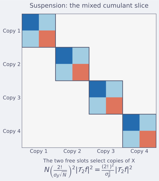
For $d=2$, the entries with one distinguished coordinate form $N$ diagonal matrix blocks. Each is scaled by $N^{-1/2}$, so their squared norms add to a quantity independent of $N$. The same disjoint-support calculation holds for higher-order tensors.

If the universal cumulant bound at order $d+1$ is $b$, then

$$|{\mathcal{T}}_{d}f|\le \frac{{\sigma }_{\beta }\sqrt{b}}{d!}.$$

Let $\beta \to \infty$, choosing a new $N$ as necessary for each $\beta$. This gives $|{\mathcal{T}}_{d}f|\le \sqrt{b}/d!$ for $f$ orthogonal to affine functions. Smooth bounded-Hessian functions with these orthogonality conditions are dense in that subspace: approximate by compactly supported smooth functions and subtract their projections onto constants and coordinates. The fixed-degree coefficient functional is continuous in $L^2$, so the bound extends by density.

For a linear function $\ell (x)=⟨v,x⟩$,

$$\begin{array}{rl}{F}_{\ell }(z)& =⟨v,\nabla {\Lambda }_{\mu }(z)⟩,\\ {\mathcal{T}}_d\ell & =\frac{1}{d!}{\kappa }_{d+1}^{\mu }(v).\end{array}$$

Now decompose an arbitrary $f=c+\ell +h$ orthogonally into its constant, linear, and remaining parts. Constants have zero positive-degree Taylor coefficients. Cauchy–Schwarz for the other two parts gives

$$|{\mathcal{T}}_{d}f{|}^2\le \frac{2b}{(d!{)}^2}\Vert f{\Vert }_2^2.$$

Taking $b=K^d(d!{)}^2$ yields

$$\begin{array}{rl}|{\mathcal{T}}_{d}f{|}^2& \le 2K^d\Vert f{\Vert }_2^2\\ & \le (2K{)}^d\Vert f{\Vert }_2^2(d\ge 2).\end{array}$$

Degree one follows directly from isotropy. The common criterion applies with $R=\sqrt{2K}$ and proves the universal Poincaré bound for regular measures. Regular approximation completes the Bizeul–Klartag–Lehec argument (Bizeul, Klartag & Lehec, 2026).

🏷️ Song–Zhang’s polynomial induction

Song–Zhang begins by obtaining dimension-free estimates at each polynomial degree:

$${\mathrm{Var}}_{\mu }(P_d^{\mu }[T])\le 1024^d(d!{)}^4|T{|}^2.$$

This is Theorem 4.1 of their second version. In the coefficient notation it says

$$c_d\le 32^{d}d!.$$

The estimate is uniform in dimension, but its extra factorial prevents direct application of the tilt-derivative criterion. Polynomial density alone cannot remove this loss: an inequality whose constants diverge with the degree does not pass to a uniform inequality for arbitrary functions.

The derivative hierarchy

Use the inverse-covariance localization above. For a fixed degree-$d$ polynomial $f$, let

$$h_j(t)={\mathbb{E}}_{{\mu }_t}{D}^{j}f$$

and let $g_j(t,x)=D^{j}f(x)-h_j(t)$. Define

$$\begin{array}{rl}& N_j(t)=\mathbb{E}⟨h_j(t),A_t^{\otimes j}{h}_j(t)⟩,\\ & V_j(t)\\ & =\mathbb{E}{\mathbb{E}}_{{\mu }_t}⟨g_j(t,X),A_t^{\otimes j}{g}_j(t,X)⟩.\end{array}$$

The outer expectation is over localization paths. Here derivatives are measured with covariance factors $A_t$, whereas cumulant slots were measured with inverse covariance factors. This is the transformation rule supplied by whitening a polynomial’s argument.

The covariance-noise estimate and Itô’s formula imply

$$N_j^{\prime }(t)\le 4j^2{N}_j(t)+9j^2{V}_j(t).$$

The cross variation between $A_t$ and $h_j(t)$ is included in this inequality. Applying lower-degree Appell bounds to the whitened posterior, and then Minkowski’s inequality over all components, gives

$$\sqrt{V_j(t)}\le \sum _{k=1}^{d-j}32^{k}k!\sqrt{N_{j+k}(t)}.$$

This is a triangular system: the fluctuations of a derivative of order $j$ are controlled by the means of its higher derivatives. There is no factor counting the number of tensor coordinates.

Closing the polynomial induction

Take $f=P_d^{\mu }[T]$, $T\ne 0$, and put

$$\begin{array}{c}Q=(d!{)}^2|T{|}^2,\\ w_j=1024^{d-j}((d-j)!{)}^2.\end{array}$$

Initially $N_j(0)=0$ for $j<d$ and $N_d(0)=Q$. If

$$M(t)=\underset{1\le j\le d}{\max }\frac{N_j(t)}{Q{w}_j},$$

then the convolution of factorial weights satisfies

$$\sum _{k=1}^s\frac{k!(s-k)!}{s!}\le 2.$$

Hence $V_j\le 4Q{w}_{j}M$ for $j<d$, while $V_d=0$. The derivative hierarchy and Gronwall give

$$M(t)\le e^{40d^{2}t}.$$

In particular, for $r=\nabla f$,

$$\begin{array}{rl}{G}_1(t)& =\mathbb{E}{\mathbb{E}}_{{\mu }_t}[r^{\mathsf{T}}{A}_{t}r]\\ & \le 5Q{w}_1{e}^{40d^{2}t}.\end{array}$$

With ${\xi }_t=A_t^{-1/2}(X-a_t)$, the posterior variance obeys

$$\begin{array}{rl}& \frac{d}{dt}\mathbb{E}{\mathrm{Var}}_{{\mu }_t}(f)\\ & =-\mathbb{E}|{\mathrm{Cov}}_{{\mu }_t}(f,{\xi }_t){|}^2.\end{array}$$

Bessel’s inequality bounds the squared covariance by the posterior variance, so $\mathbb{E}{\mathrm{Var}}_{{\mu }_{\tau }}(f)\ge e^{-\tau }{\mathrm{Var}}_{\mu }(f)$.

At time $\tau$, the posterior has curvature matrix $Q_{\tau }={\int }_0^{\tau }{A}_s^{-1}ds$. The matrix Brascamp–Lieb inequality gives

$${\mathrm{Var}}_{{\mu }_{\tau }}(f)\le {\mathbb{E}}_{{\mu }_{\tau }}[r^{\mathsf{T}}{Q}_{\tau }^{-1}r].$$

The needed comparison between the accumulated precision and covariance is

$$Q_{\tau }^{-1}⪯{\tau }^{-2}{\int }_0^{\tau }{A}_{s}ds.$$

It follows from the exact nonnegative remainder, valid for every vector $v$,

$$\begin{array}{c}\begin{array}{rl}& {\int }_0^{\tau }{v}^{\mathsf{T}}{A}_{s}vds-{\tau }^2{v}^{\mathsf{T}}{Q}_{\tau }^{-1}v\\ & ={\int }_0^{\tau }|{\zeta }_s{|}^{2}ds,\end{array}\\ \begin{array}{rl}{\zeta }_s& =A_s^{1/2}v\\ & -\tau A_s^{-1/2}{Q}_{\tau }^{-1}v.\end{array}\end{array}$$

For $s\le \tau$, the martingale tower identity applies to each fixed entry of $r{r}^{\mathsf{T}}$, with the random matrix $A_s$ held fixed at time $s$. Therefore

$${\mathrm{Var}}_{\mu }(f)\le \frac{e^{\tau }}{{\tau }^2}{\int }_0^{\tau }{G}_1(s)ds.$$

Choosing $\tau =(40d^2{)}^{-1}$ bounds the exponential factor and yields

$$\begin{array}{rl}{\mathrm{Var}}_{\mu }(f)& \le 600d^{2}Q{w}_1\\ & \le 1024^d(d!{)}^4|T{|}^2.\end{array}$$

Degree one is isotropy. Conditioning on expanding balls, recentering, and whitening removes compact support; only moments through degree $2d$ are needed at this stage (Song & Zhang, 2026a, sec.4).

🏷️ From polynomial coefficients to curvature estimates

The general form of the analytic comparison retains a degree-dependent coefficient profile. Let $\nu$ be centered and regular with covariance at most $I$, and let its potential satisfy $D^{2}W⪰aI$, where $0<a\le 1$. Suppose that $\ell :\mathbb{N}\to [1,\infty )$ is nondecreasing and

$$c_k(\nu )\le R^k\frac{\ell (k{)}^k}{(k+1{)}^2}(k\ge 1),$$

with $R$ above a universal threshold. Then, for every dyadic $d\ge 2$,

$$C_P(\nu )\le C{R}^2\ell (d{)}^2{a}^{-1/(d+1)}.$$

This is the fixed-accuracy form of Song–Zhang, Theorem 5.1. The degree $d$ and the curvature $a$ play separate roles: increasing $d$ weakens the curvature penalty but exposes a potentially larger polynomial coefficient.

The inverse-gradient families, Bochner decrease, and partial symmetrization introduced above underlie this theorem. Song–Zhang uses an $H^{-1/2}$ normalization that tracks both the $L^2$ mass and the energy of each family. For a centered family $u$, set

$$\begin{array}{c}\beta =\frac{\Vert u{\Vert }_2^2}{\Vert H^{-1/2}u{\Vert }_2^2},\\ h=\sqrt{\beta }{H}^{-1/2}u.\end{array}$$

Then $\Vert h{\Vert }_2=\Vert u{\Vert }_2$, and the nonnegative defect

$$\chi =\Vert H^{1/2}u{\Vert }_2^2-\beta \Vert u{\Vert }_2^2$$

satisfies the exact identity

$$\Vert \nabla (H^{-1/2}h-{\beta }^{-1/2}u){\Vert }_2^2=\chi /\beta .$$

That identity permits symmetry errors to be charged to energy decrease. The common scalar normalizer applies to the entire tensor family, preserving the summed identities.

For the initial estimate $c_k\le 32^{k}k!$, take $\ell (k)=k$ and enlarge $R$ to absorb $(k+1{)}^2$. Then

$$C_P(\nu )\lesssim d^2{a}^{-1/(d+1)}.$$

Choose a dyadic $d$ comparable to $\log (e+a^{-1})$. Since

$$a^{-1/(d+1)}=\exp \left(\frac{\log (a^{-1})}{d+1}\right),$$

the curvature penalty is bounded, giving

$$C_P(\nu )\lesssim [\log (e+a^{-1}){]}^2.$$

Feeding a curvature estimate back into polynomial bounds

The next localization argument uses the newly improved Poincaré estimate for each posterior. A useful affine extension makes this possible without assuming scalar covariance or commuting matrices.

Suppose $\Phi (a)$ bounds the Poincaré constant for every centered regular law with covariance at most $I$ and curvature at least $aI$. If a posterior has covariance $A\succ 0$ and curvature matrix $B\succ 0$, put $M=A+\delta B^{-1}$. Then

$$\begin{array}{rl}& {\mathrm{Var}}_{\nu }(f)\\ & \le \Phi (\delta ){\mathbb{E}}_{\nu }⟨M\nabla f,\nabla f⟩.\end{array}$$

Indeed, the transformation $M^{-1/2}(X-\mathbb{E}X)$ has covariance at most $I$. Also $M⪰\delta B^{-1}$ implies $M^{1/2}B{M}^{1/2}⪰\delta I$. Apply the profile to this transformed law and use the chain rule. Regular approximation supplies the same estimate for nonsmooth posteriors.

Write

$$\begin{array}{rl}{\ell }_0(x)& =x,\\ {\ell }_{r+1}(x)& =\log (e+{\ell }_r(x)).\end{array}$$

Song–Zhang, Theorem 6.3, proves the following transfer: if the whole class satisfies

$$C_P(\nu )\le {\Gamma }^2{\ell }_r(a^{-1}{)}^2,$$

then its Appell coefficients satisfy

$$c_d\le (2^{12}\Gamma {)}^d\frac{{\ell }_r(d{)}^d}{(d+1{)}^2}.$$

The derivative hierarchy is the same as before, now with weights proportional to ${\ell }_r(k{)}^k/(k+1{)}^2$. The denominator makes their convolution uniformly bounded:

$$\sum _{k=1}^s\frac{(s+1{)}^2}{(k+1{)}^2(s-k+1{)}^2}\le 16.$$

Localization time remains of order $d^{-2}$. The logarithmic profile absorbs this change of scale because ${\ell }_r(C{d}^2)\lesssim {\ell }_r(d)$ uniformly in $r\ge 1$. Feeding the resulting coefficients into the curvature theorem introduces another logarithm in $a^{-1}$.

Repeated improvement of the logarithm is only part of the proof. The constants also need to remain controlled as the number of refinements grows.

🏷️ Repeated refinements and their cumulative cost

The technical block constructions in Song–Zhang are designed to control losses from centering and from imperfect tensor symmetry over many inverse-gradient iterations. The relevant blocks are finite stretches of these iterations, with a chosen starting family. Their order determines how small the starting loss is as a function of an operator scale.

The remaining exposition states the quantitative block results used in the proof and explains their final induction. The proofs of all the intermediate block-extension lemmas in Sections 6, 8, and 9 of the 140-page paper are not reproduced here.

Inner depth, polynomial degree, and block order

The first optimized refinement gives

$$\begin{array}{c}{C}_P(\nu )\le C(r+1{)}^{1/3}{\ell }_r(a^{-1}{)}^2,\\ r\ge 1.\end{array}$$

This is Proposition 6.1. Its cubic cost comes from starting blocks whose mass loss and excess energy are of order $z^{-3}$ at a suitable squared operator scale $z$. Fitting this loss into a budget of order $(r+1{)}^{-1}$ produces the factor $(r+1{)}^{1/3}$.

At depth comparable to $1+{\log }^{\ast }(a^{-1}+2)$, the iterated logarithm is universally bounded. This gives a log-star curvature bound, but still leaves dependence on $a$ through the depth factor.

For comparison with dimension bounds, the paper also uses Gaussian localization with quadratic penalty $t|x{|}^2/2$. At time $t\asymp 1/\log (en)$, its controlled-covariance posteriors preserve enough of a Poincaré witness’s variance to transfer the curvature estimate back. The resulting intermediate theorem is

$$\begin{array}{rl}{C}_P(\mu )& \lesssim [1+{\log }^{\ast }(n+2){]}^{1/3},\\ {\psi }_n& \lesssim [1+{\log }^{\ast }(n+2){]}^{1/6}.\end{array}$$

This is Theorem 7.1 in v2. The final proof continues to use the full family of curvature estimates at all allowed depths, rather than only this optimized dimensional consequence.

Higher odd block orders $Q$ replace the cubic starting loss by an order-$z^{-Q}$ loss, with quantitatively controlled constants. This changes the depth cost to $(r+1{)}^{1/Q}$. A choice $Q$ comparable to $\log (r+1)$ can keep that factor bounded, subject to the construction’s depth thresholds.

There are therefore three distinct parameters:

Parameter	Role
Polynomial degree $d$	Makes the curvature exponent $1/(d+1)$ small
Inner depth $r$	Counts compositions of $x\mapsto \log (e+x)$
Odd block order $Q$	Controls the cost of carrying out a refinement to depth $r$

An outer refinement extracts better polynomial coefficients by choosing $r$ separately at each degree, then repeats the entire argument with those coefficients.

Why repeated log-star improvement is still insufficient

Set

$$\begin{array}{c}\mathfrak{t}(x)=1+{\log }^{\ast }(x+2),\\ {\mathfrak{t}}_j={\mathfrak{t}}^{\circ j}.\end{array}$$

For a fixed odd order $q\ge 3$, Section 8 obtains bounds of the form

$$C_P(\nu )\le C_q{C}_{\ast }^{j-1}{\mathfrak{t}}_j(1+a^{-1}{)}^{1/q}.$$

For each fixed $a$, finitely many outer rounds make the height term bounded. But the required number

$$\kappa (x)=\min \{j\ge 0:{\mathfrak{t}}_j(x)\le 3\}$$

is unbounded as $x\to \infty$. Therefore the accumulated factor $C_{\ast }^{\kappa (x)}$ cannot be called a universal constant. Section 9 replaces this fixed cost per repetition by losses approaching one, while controlling the increased parameter thresholds that such accuracy demands.

One coefficient radius throughout the refinements

Define the common coefficient radius

$$\mathcal{A}(\mu )=\max \left\{1,\underset{d\ge 2}{\sup }{c}_d(\mu {)}^{2/(d-1)}\right\}.$$

For a fixed regular measure this is finite. To see the mechanism, let $\mathcal{U}={\nabla }_0{H}^{-1}$ act into the direct sum over derivative coordinates, and put $R_{\mathrm{res}}=\Vert \mathcal{U}{\Vert }_{\mathrm{op}}^2$. The integration-by-parts identity for the polynomial tests gives

$$c_d\le \sqrt{R_{\mathrm{res}}}{c}_{d-1},c_1\le 1.$$

Also $R_{\mathrm{res}}\le {\lambda }^{-1}<\infty$ by the inverse-energy inequality. Thus $\mathcal{A}\le \max \{1,R_{\mathrm{res}}\}$ for this measure, without yet asserting a universal bound.

The curvature theorem, applied with a constant coefficient profile and then $d\to \infty$ through dyadic values, gives

$$C_P(\mu )\le 2^{85}\mathcal{A}(\mu ).$$

The large numerical factor in Song–Zhang, Lemma 8.18, is universal and is not optimized. The proof estimates $\mathcal{A}$ directly during the later refinements, paying this comparison factor only once at the end.

Retaining earlier coefficient bounds

Making one outer round cost $e^{C\epsilon }$ requires a degree cutoff of size

$$K_{\epsilon }=\lceil C_{\mathrm{cut}}{\epsilon }^{-2}\rceil .$$

Smaller losses therefore leave a larger initial range of degrees requiring separate control. The construction retains earlier coefficient bounds $c_k\le {\mathcal{H}}_i(k{)}^{k-1}$ and assigns them to consecutive ranges. These bounds are kept fixed during the new induction; they are already established estimates, not assumptions about its desired conclusion.

A decisive estimate makes the constants independent of the number of retained bounds. If the error on a range has damping $e^{-c{\alpha }_{i}k}$ and that range begins beyond $K_i\ge C_{\mathrm{cut}}{\alpha }_i^{-2}$, then

$${\alpha }_{i}k\ge \sqrt{C_{\mathrm{cut}}k}.$$

Summing over all disjoint ranges is therefore bounded by a single convergent tail

$$\sum _{k>K_0}{k}^M{e}^{-c^{\prime }\sqrt{C_{\mathrm{cut}}k}}.$$

The exponent $M$ is one of finitely many fixed exponents needed by the block estimates. Bounding each range by a separate constant and then adding those constants would lose uniformity in the number of refinements. Proposition 9.23 instead uses the single degree sum to obtain bounds valid for an arbitrary finite list of inherited estimates.

Contracting the remaining height dependence

Define $\chi (x)=\max \{3,1+\kappa (x)\}$. The discontinuous height functions are replaced by forward averages

$$\begin{array}{rl}& \overline{f}(x)\\ & =\max \left\{4,\frac{1}{4}{\int }_0^{4}f(x+t)dt\right\},\\ & f\in \{\mathfrak{t},\chi \}.\end{array}$$

On $[1,\infty )$ their jumps have size at most one and are spaced sufficiently far apart that $0\le f(x+4)-f(x)\le 1$. Consequently the derivative of the average, wherever it exists, lies in $[0,1/4]$. The averaged maps are nondecreasing $1/4$-Lipschitz majorants, with a constant floor at four.

Put

$$W_i(x)=\overline{\mathfrak{t}}({\overline{\chi }}^{\circ i}(x)).$$

Then $W_i$ is $4^{-i-1}$-Lipschitz. More useful than applying that Lipschitz constant directly to a very large argument is the fixed-power estimate

$$W_i(C{x}^p)\le W_i(x)+b_{C,p}{4}^{-i}.$$

The first height map absorbs the power into a bounded additive change, and the subsequent maps contract that change. Products and sums admit corresponding estimates. These are the scalar estimates in Lemmas 9.17–9.18.

The iteration reaches the constant floor in finitely many steps for each fixed argument. Indeed, $\overline{\chi }$ contracts toward four and equals four throughout $[4,6]$; after finitely many contractions the argument enters that interval.

The final quantitative induction

The smoothed logarithms ${\ell }_r(x)$ converge, as $r\to \infty$, to the positive fixed point $\varrho$ of $\varrho =\log (e+\varrho )$. Normalize them by

$${\mathcal{L}}_r(x)={\ell }_r(x)/\varrho .$$

This allows their limiting factor to be one. A fixed factor larger than one at each repetition would defeat summability.

Choose

$$\begin{array}{rl}{\alpha }_i& =\frac{1}{16}{2}^{-i},\\ R_i& =\lceil C_R{\alpha }_i^{-12}\rceil ,\\ A_{i+1}& =e^{C_A{\alpha }_i}{A}_i,\\ S_0& =1,S_{i+1}=S_i+B{2}^{-i}.\end{array}$$

The $R_i$ here are thresholds for the allowed inner depth. Proposition 9.25 proves, for every finite $i$, every $r\ge R_i$, and every regular law in the covariance-normalized class,

$$\mathcal{A}(\mu )\le A_i[W_i(r)+S_i{]}^{1/3}{\mathcal{L}}_r(a^{-1}{)}^2.$$

The amplitude, additive offset, and threshold have all been kept explicit. Two geometric series immediately give

$$A_i\le A_0{e}^{2C_A{\alpha }_0},S_i\le 1+2B.$$

For the transition from $i$ to $i+1$ at a prescribed depth $r$, take

$$j=\kappa (r),\epsilon =\frac{{\alpha }_i}{j+1}.$$

Perform $j$ outer rounds, so the product of their losses is at most $e^{C\epsilon j}\le e^{C{\alpha }_i}$. Choose an admissible odd block order with

$$Q\gtrsim \max \{{\epsilon }^{-4},{\alpha }_i^{-1}\log (r+1)\}.$$

Then $(r+1{)}^{1/Q}\le e^{{\alpha }_i}$. The polynomial threshold $r\ge R_{i+1}$ makes this choice compatible with the lower bounds on depth. The new height penalty is controlled by

$$W_i({\epsilon }^{-1})\le W_{i+1}(r)+C{2}^{-i}.$$

These estimates produce exactly the multiplicative and additive increments allowed in $A_{i+1}$ and $S_{i+1}$. The finite list of earlier coefficient bounds controls the degree ranges exposed by the smaller $\epsilon$.

One remaining issue is that $R_i$ itself grows exponentially in $i$. Lemma 9.24 proves

$$W_i(R_i+C\mathfrak{t}(x))\le W_i(x)+b{2}^{-i}.$$

The fixed-power estimate is used before contraction. In particular,

$$\begin{array}{rl}{W}_i(C{\alpha }_i^{-p})& \le W_i(2^i)+b_{C,p}{4}^{-i}\\ & \le 4+b_{C,p}^{\prime }{2}^{-i}.\end{array}$$

Directly multiplying $R_i$ by the Lipschitz constant would not give this bound; absorbing its fixed power first is necessary.

For the final choice, fix the measure and set $x=\max \{1,a^{-1}\}$. Choose a finite $i$ with $W_i(x)=4$, and then choose the allowed depth

$$r=R_i+\lceil C\mathfrak{t}(x)\rceil .$$

The threshold estimate bounds $W_i(r)$ universally, and the choice of $r$ bounds ${\mathcal{L}}_r(a^{-1})$ universally. The bounded amplitudes and offsets now give

$$\mathcal{A}(\mu )\le C,C_P(\mu )\le C.$$

Every degree, depth, and number of rounds used for a fixed regular law is finite. Their values may depend on that law’s curvature; the resulting constant does not. Applying the universal inequality to each regular approximation and passing the inequality itself to the limit completes Song–Zhang’s proof (Song & Zhang, 2026a).

🏷️ Consequences and comparison of the mechanisms

The two arguments reach the same spectral statement through different ways of controlling the full sequence of polynomial coefficients.

Ingredient	Cumulant and suspension argument	Polynomial refinement argument
Initial geometric estimate	Quadratic-form variance bound	Same quadratic-form variance bound
Quantity propagated by localization	Cumulant slices in the inverse covariance metric	Expected polynomial derivatives in the covariance metric
Main normalization	$((m-1)!{)}^2$ for squared cumulant slices	$d!$ in $c_d=\sqrt{K_d}/d!$
Passage to arbitrary functions	Encode an observable as a new coordinate	Control the common coefficient radius at every degree
Removal of the remaining loss	Exact factorial cancellation and cancellation across independent copies	Summable multiplicative and additive refinement costs
Spectral mechanism	Song–Zhang tilt-derivative criterion	Polynomial-to-curvature comparison and the coefficient radius

The resulting Poincaré inequality implies exponential concentration for Lipschitz functions, with universal constants in isotropic position. In particular, for a centered 1-Lipschitz observable,

$$\mathbb{P}(|f(X)|\ge t)\le 2e^{-ct}$$

after choosing a universal $c>0$. This is exponential concentration; log-concavity and KLS do not force Gaussian tails. A centered exponential variable already illustrates the distinction.

For the squared radius, $\nabla |x{|}^2=2x$, and isotropy gives

$$\mathrm{Var}(|X{|}^2)\le 4C_P(\mu )\mathbb{E}|X{|}^2\le 4Cn.$$

Moreover,

$$\begin{array}{rl}(|X|-\sqrt{n}{)}^2& =\frac{(|X{|}^2-n{)}^2}{(|X|+\sqrt{n}{)}^2}\\ & \le \frac{(|X{|}^2-n{)}^2}{n}.\end{array}$$

so the radial fluctuations have bounded squared mean. This recovers a thin-shell bound, but does not recover the sharp constant $8$ in the quadratic input. That sharp input was already used to start both arguments.

The dimension-free isoperimetric bound also improves the conductance estimates underlying sampling and volume algorithms. A complete running-time statement still depends on the walk, its step size, the initial distribution, and the computational access to the density; the spectral theorem by itself does not specify those choices.

Several logical distinctions carry the proofs. A bound for quadratic forms starts the process, but all degrees are needed. Control of each directional cumulant is weaker than control of a whole Hilbert–Schmidt slice. A finite number of refinements for each dimension is compatible with an unbounded total cost. In the cumulant proof, the exact factorial identity resolves the degree growth; in the polynomial proof, the geometric loss budgets resolve the refinement growth. The common analytic criterion then turns these quantitative estimates into the universal spectral gap.

Links

• on a sharp quadratic-form inequality and the KLS constant develops the moment-map and matrix-energy proof of the sharp quadratic estimate that supplies the third-cumulant bound.
• on Eldan’s stochastic localization and the KLS conjecture introduces the measure-valued martingale, covariance evolution, and the passage from localized curvature to isoperimetry.
• on an almost constant lower bound in the KLS conjecture explains Chen’s earlier recursive improvements and provides a comparison with the refinement of coefficient and curvature estimates here.
• on KLS localization lemma treats the classical reduction to one-dimensional needles, a different form of localization underlying the earlier theory.

📚 References

🐻  Bizeul, P., Klartag, B. & Lehec, J. 2026. Presenting a proof of the Kannan–Lovasz–Simonovits conjecture.

🐻  Letwin, B. 2026. The KLS Constant Is O(\log^1/4 n).

🐻  Song, Z. & Zhang, X. 2026a. An O(1) Bound for the KLS Constant.

🐻  Song, Z. & Zhang, X. 2026b. An O(4^{\log^* n}) Bound for the KLS Constant.