Strong convergence through rational trace expansions

Overview

Convergence of the average eigenvalue distribution does not exclude a few exceptional eigenvalues. Strong convergence asks for convergence of the operator norm of every fixed noncommutative polynomial in a family of random matrices. Chen, Garza-Vargas, Tropp, and van Handel develop a method that obtains this much stronger conclusion from rational formulas for expected traces and information about their first few asymptotic coefficients (Chen et al., 2026).

The argument combines polynomial interpolation, the Markov inequality for derivatives, Chebyshev expansions, and the support theory of distributions. For random permutations, the remaining combinatorics concerns words that are proper powers in a free group. Applications include an effective Friedman theorem, a staircase of rare-event probabilities for regular graphs, and strong convergence for stable representations of symmetric groups.

The source is A new approach to strong convergence, arXiv:2405.16026v3, revised February 11, 2025, and published in Annals of Mathematics 203 (2026), 555–602. References to sections and numbered results below use the arXiv version. We develop the analytic argument and its combinatorial implementation, while stating explicitly the external factorization and word-measure theorems on which the general applications depend.

🏷️ Matrices, traces, and the outlier problem

For a matrix $X$ acting on ${\mathbb{C}}^n$, its operator norm is

$$\Vert X\Vert =\underset{\Vert v{\Vert }_2=1}{\sup }\Vert Xv{\Vert }_2.$$

If $X=X^{\ast }$ is self-adjoint, the spectral theorem gives real eigenvalues ${\lambda }_1,\dots ,{\lambda }_n$ and

$$\begin{array}{rl}\Vert X\Vert & =\underset{j}{\max }|{\lambda }_j|,\\ {\mathrm{tr}}_{n}h(X)& =\frac{1}{n}\mathrm{Tr}h(X)\\ & =\frac{1}{n}\sum _{j=1}^{n}h({\lambda }_j).\end{array}$$

Here $h(X)$ is defined by applying $h$ to the eigenvalues, and $\mathrm{Tr}$ denotes the ordinary, unnormalized trace. Thus normalized traces describe the empirical spectral measure

$${\mu }_X=\frac{1}{n}\sum _{j=1}^n{\delta }_{{\lambda }_j}.$$

For uniformly bounded self-adjoint matrices, convergence of all expected moments implies weak convergence of their expected empirical measures. Indeed, polynomials approximate continuous functions uniformly on a common compact interval. This statement concerns averages over eigenvalues; an individual eigenvalue has mass only $1/n$.

An outlier invisible to the limiting moments

Let $X^N=\mathrm{diag}(2,0,\dots ,0)$. For every positive integer $p$,

$${\mathrm{tr}}_N(X^N{)}^p=\frac{2^p}{N}⟶0,$$

while $\Vert X^N\Vert =2$ for every $N$. The empirical measures converge to ${\delta }_0$, but the norm does not converge to the norm of the zero operator.

The distinction persists for random matrices. To rule out an outlier, one needs an estimate fine enough to detect a single eigenvalue, rather than just a vanishing fraction of the spectrum.

Noncommutative polynomials

A noncommutative $\ast$-polynomial is a finite linear combination of words in formal variables $z_1,\dots ,z_d,z_1^{\ast },\dots ,z_d^{\ast }$. Order matters: $z_1{z}_2$ and $z_2{z}_1$ are different words. For example,

$$P(z,z^{\ast })=z_1{z}_2+z_2^{\ast }{z}_1^{\ast }$$

is self-adjoint upon evaluation on any tuple of matrices. More generally, we allow matrix coefficients:

$$\begin{array}{c}P(z,z^{\ast })=\sum _w{A}_w\otimes w(z,z^{\ast }),\\ A_w\in M_D(\mathbb{C}).\end{array}$$

The tensor product means that $A_w$ acts on a coefficient space ${\mathbb{C}}^D$, while the word acts on the original matrix space. The degree $q_0$ is the maximum word length in the chosen polynomial expression.

A family ${\mathbf{X}}^N$ converges strongly in probability to a tuple of bounded operators $\mathbf{x}$ when, for every fixed such polynomial,

$$\Vert P({\mathbf{X}}^N,{\mathbf{X}}^{N\ast })\Vert \stackrel{\mathbb{P}}{\to }\Vert P(\mathbf{x},{\mathbf{x}}^{\ast })\Vert .$$

The scalar-coefficient definition is obtained with $D=1$; the results here also cover each fixed $D$. This is a statement about norms of polynomial evaluations, not convergence in the strong operator topology on a common Hilbert space.

It suffices to prove the result for self-adjoint polynomials, since

$$\Vert P{\Vert }^2=\Vert P^{\ast }P\Vert .$$

For quantitative estimates one must remember that $P^{\ast }P$ has degree at most $2q_0$, and that an error in a squared norm is not the same as an error in the norm itself.

🏷️ Permutation matrices and their free limit

Let ${\sigma }_1,\dots ,{\sigma }_d$ be independent uniform permutations of $\{1,\dots ,N\}$. Their permutation matrices act by

$${\overline{S}}_i^N{e}_j=e_{{\sigma }_i(j)}.$$

They are unitary, with $({\overline{S}}_i^N{)}^{\ast }=({\overline{S}}_i^N{)}^{-1}$. Every permutation fixes the all-ones vector $1_N$, so we restrict to the common invariant subspace

$$\begin{array}{c}{H}_N=\{v\in {\mathbb{C}}^N:⟨1_N,v⟩=0\},\\ S_i^N={\overline{S}}_i^N{|}_{H_N}.\end{array}$$

Removing this one-dimensional representation is essential. Otherwise the polynomial ${\sum }_i(z_i+z_i^{\ast })$ always has eigenvalue $2d$, which exceeds the limiting tree norm when $d\ge 2$.

We follow the paper’s convenient normalization

$${\mathrm{tr}}_{N}T=\frac{1}{N}{\mathrm{Tr}}_{H_N}T,$$

even though $\dim H_N=N-1$. In particular,

$${\mathrm{tr}}_N{I}_{H_N}=1-\frac{1}{N}.$$

For matrix coefficients, ${\mathrm{tr}}_{DN}$ similarly means $\mathrm{Tr}/(DN)$ on ${\mathbb{C}}^D\otimes H_N$. This convention will contribute a genuine first-order correction.

Reduced words and the free group

The free group ${\mathbb{F}}_d$ consists of reduced words in $g_1,\dots ,g_d,g_1^{-1},\dots ,g_d^{-1}$. Reduction deletes adjacent inverse pairs. Multiplication concatenates words and then reduces them. The identity $e$ is the empty word. For example,

$$\begin{array}{c}{g}_1{g}_2{g}_2^{-1}{g}_1=g_1^2,\\ g_1{g}_2{g}_1^{-1}{g}_2^{-1}\ne e.\end{array}$$

There are no relations beyond inverse cancellation. Its Cayley graph, with one edge for multiplication by each generator or inverse, is the infinite $2d$-regular tree.

The Hilbert space ${\ell }^2({\mathbb{F}}_d)$ has orthonormal basis $\{{\delta }_w:w\in {\mathbb{F}}_d\}$. The left regular representation is

$$\lambda (g){\delta }_w={\delta }_{gw},s_i=\lambda (g_i).$$

Each $s_i$ is unitary. The limiting trace is

$$\tau (T)=⟨{\delta }_e,T{\delta }_e⟩.$$

For a group element $w$,

$$\tau (\lambda (w))=1_{\{w=e\}}.$$

Thus the trace extracts the coefficient of the identity. On the norm-closed algebra generated by the $s_i$, it is positive, normalized, and tracial: $\tau (A^{\ast }A)\ge 0$, $\tau (I)=1$, and $\tau (AB)=\tau (BA)$. The trace identity follows first for group elements, because $uv=e$ exactly when $vu=e$, and then by linearity and continuity.

This trace is also faithful: $\tau (A^{\ast }A)=0$ implies $A=0$. Indeed, the equality gives $A{\delta }_e=0$. Left translations commute with right translations, and every basis vector is a right translate of ${\delta }_e$. Hence $A$ annihilates every basis vector.

The operators $s_1,\dots ,s_d$ are called free Haar unitaries. For this post their explicit construction is enough. The familiar freeness condition can also be seen directly: an alternating product of centered polynomials in different individual generators expands into nonempty reduced words and therefore has trace zero.

Two different norms

For a polynomial $P$, put

$$\begin{array}{rl}{X}_N& =P({\mathbf{S}}^N,{\mathbf{S}}^{N\ast }),\\ X_F& =P(\mathbf{s},{\mathbf{s}}^{\ast }),\\ R& =\Vert X_F\Vert ,\\ K& =\underset{\mathbf{U}}{\sup }\Vert P(\mathbf{U},{\mathbf{U}}^{\ast })\Vert .\end{array}$$

The supremum is over unitary tuples of all finite dimensions. It is the full free-group $C^{\ast }$-norm, whereas $R$ is the reduced norm. In particular,

$$\begin{array}{c}R\le K\le \sum _w\Vert A_w\Vert ,\\ \Vert X_N\Vert \le K.\end{array}$$

The scalar bound on the right is useful even when $K$ is hard to compute. The analytic estimates work with any known common bound on the polynomial evaluations; the paper states its main results with the exact full norm.

The distinction between $K$ and $R$ is central: $K$ bounds every possible realization, while $R$ describes the limiting edge. The method must exclude the interval between them with high probability.

🏷️ The regular tree and its spectral edge

Write $r=2d$ and $b=r-1$. The adjacency operator of the infinite $r$-regular tree is

$$A_F=\sum _{i=1}^d(s_i+s_i^{\ast }).$$

Its norm is

$$\Vert A_F\Vert =2\sqrt{r-1}=2\sqrt{b}.$$

Here is a direct proof of the edge value. Orient the tree toward a fixed end at infinity, so every vertex has one parent and $b$ children. Let

$$(Tf)(v)=\sum _{u:u\text{ is a child of }v}f(u).$$

Cauchy–Schwarz gives $\Vert Tf{\Vert }_2^2\le b\Vert f{\Vert }_2^2$, because each vertex belongs to exactly one child set. Since $A_F=T+T^{\ast }$,

$$\Vert A_F\Vert \le 2\sqrt{b}.$$

For the reverse inequality, fix a root $o$ and use the finitely supported radial vector

$$f_L(v)=b^{-\mathrm{dist}(o,v)/2}{1}_{\{\mathrm{dist}(o,v)\le L\}}.$$

There are $r{b}^{j-1}$ vertices at distance $j\ge 1$. Counting vertices and edges therefore gives

$$\begin{array}{rl}\Vert f_L{\Vert }_2^2& =1+\frac{rL}{b},\\ ⟨f_L,A_F{f}_L⟩& =\frac{2rL}{\sqrt{b}}.\end{array}$$

Their ratio tends to $2\sqrt{b}$, proving equality.

The root spectral measure is the Kesten–McKay measure, with density

$$\begin{array}{c}{\rho }_r(x)=\frac{r\sqrt{4(r-1)-x^2}}{2\pi (r^2-x^2)},\\ |x|<2\sqrt{r-1},\end{array}$$

and zero outside this interval. For completeness, this density follows from a resolvent recursion. With the convention $(z-A{)}^{-1}$, the root Green function $h(z)$ of a forward branch and the full root Green function $G(z)$ satisfy

$$\begin{array}{rl}h(z)& =\frac{1}{z-bh(z)},\\ h(z)& =\frac{z-\sqrt{z^2-4b}}{2b},\\ G(z)& =\frac{1}{z-rh(z)}.\end{array}$$

Choose the square-root branch with $h(z)\sim 1/z$ at infinity. Taking $-{\pi }^{-1}\mathrm{Im}G(x+i0)$ yields the displayed density.

For the corresponding finite permutation model,

$$\begin{array}{rl}{\overline{A}}_N& =\sum _{i=1}^d({\overline{S}}_i^N+{\overline{S}}_i^{N\ast }),\\ A_N& ={\overline{A}}_N{|}_{H_N}.\end{array}$$

This is a regular multigraph: loops and multiple edges are allowed, and a loop contributes two to the adjacency diagonal and to the degree. Its constant eigenvector has eigenvalue $r$. The norm $\Vert A_N\Vert$ is the largest absolute value among the remaining eigenvalues. In this example,

$$K=2d,R=2\sqrt{2d-1}.$$

The gap between these numbers is exactly the gap strong convergence must close.

🏷️ The quantitative conclusions

Throughout the quantitative statements, $d\ge 2$, the polynomial is fixed and self-adjoint, and $0<\epsilon <K-R$. We write $a\lesssim b$ for an inequality with a universal multiplicative constant.

Strong convergence of permutation matrices

For a self-adjoint polynomial $P$ of degree $q_0\ge 1$ with coefficients in $M_D(\mathbb{C})$,

$$\begin{array}{rl}& \mathbb{P}\{\Vert X_N\Vert \ge R+\epsilon \}\\ & \lesssim \frac{D}{N}{\left(\frac{K{q}_0\log d}{\epsilon }\right)}^8\\ & \cdot \log \left(\frac{eK}{\epsilon }\right).\end{array}$$

Together with the lower bound proved below, this yields $\Vert X_N\Vert \to R$ in probability (Chen et al., 2026, sec.3.3).

For fixed $P,d,D$, the positive excess over $R$ is therefore

$$\begin{array}{rl}& (\Vert X_N\Vert -R{)}_{+}\\ & =O_{\mathbb{P}}\left({\left(\frac{\log N}{N}\right)}^{1/8}\right).\end{array}$$

Here $O_{\mathbb{P}}(a_N)$ means that the quantity divided by $a_N$ is bounded in probability. To see the rate, substitute $\epsilon =M(\log N/N{)}^{1/8}$ into the probability bound. Its limsup is at most a constant times $M^{-8}$.

This is a quantitative upper error estimate; the lower-bound argument below gives convergence without this rate. Also, an $O(N^{-1})$ failure probability is not summable over all $N$, so this estimate alone does not imply almost sure convergence.

Effective Friedman theorem

For the permutation model of a random $2d$-regular graph,

$$\begin{array}{rl}& \mathbb{P}\{\Vert A_N\Vert \ge 2\sqrt{2d-1}+\epsilon \}\\ & \lesssim \frac{1}{N}{\left(\frac{d\log d}{\epsilon }\right)}^8\log \left(\frac{2ed}{\epsilon }\right),\end{array}$$

for $0<\epsilon <2d-2\sqrt{2d-1}$ (Chen et al., 2026, sec.3.2).

The point of this bound is its derivation by a method that also works for arbitrary polynomials. It is not the optimal edge-fluctuation scale for regular graphs.

If $P$ is constant, its norm is independent of $N\ge 2$ and there is nothing to prove. If $K=R$, the deterministic inequality $\Vert X_N\Vert \le R$ already supplies the upper bound. These cases should be separated before using a formula requiring $0<\epsilon <K-R$.

🏷️ Why the direct moment method becomes difficult

For self-adjoint $X_N$ acting on a space of dimension at most $DN$,

$$\Vert X_N{\Vert }^{2p}\le \mathrm{Tr}{X}_N^{2p}.$$

Suppose, for a fixed $p$, that the normalized expected trace converges to the free trace. Since the latter is at most $R^{2p}$, this suggests

$$\begin{array}{rl}& (\mathbb{E}\Vert X_N{\Vert }^{2p}{)}^{1/(2p)}\\ & \le (DN{)}^{1/(2p)}(R+o(1)).\end{array}$$

The factor $(DN{)}^{1/(2p)}$ disappears only when $p\gg \log N$ for fixed $D$. Fixed-degree moment asymptotics say nothing uniform in that range.

There is also a genuine obstruction. If an event with $\Vert X_N\Vert \ge R+\eta$ has probability at least $N^{-c}$, then

$$\mathbb{E}\mathrm{Tr}{X}_N^{2p}\ge N^{-c}(R+\eta {)}^{2p}.$$

For $p/\log N\to \infty$, its ratio to $N{R}^{2p}$ diverges when $R>0$. Rare exceptional configurations can dominate very high moments while their probability still tends to zero. In regular graphs, finite dense configurations called tangles cause precisely this behavior.

The new argument retains the trace information but applies it to functions bounded on the whole deterministic interval $[-K,K]$. Linear combinations of moments can preserve cancellations that disappear when individual monomials are bounded separately.

🏷️ Smooth spectral detectors and correction distributions

Suppose one can establish, for every smooth $h$, an expansion

$$\begin{array}{rl}& \mathbb{E}{\mathrm{tr}}_{DN}h(X_N)\\ & ={\nu }_0(h)+\frac{{\nu }_1(h)}{N}+O_h(N^{-2}),\end{array}$$

where

$${\nu }_0(h)=({\mathrm{tr}}_D\otimes \tau )(h(X_F)).$$

Choose a smooth detector $\chi :\mathbb{R}\to [0,1]$ satisfying

$$\{\begin{array}{ll}\chi (x)=0,& |x|\le R+\epsilon /2,\\ \chi (x)=1,& |x|\ge R+\epsilon .\end{array}$$

If both ${\nu }_0$ and ${\nu }_1$ vanish on this detector, then

$$\begin{array}{rl}& \mathbb{P}\{\Vert X_N\Vert \ge R+\epsilon \}\\ & \le \mathbb{E}\mathrm{Tr}\chi (X_N)\\ & =DN\mathbb{E}{\mathrm{tr}}_{DN}\chi (X_N)\\ & =O_{\chi }(D/N).\end{array}$$

The first inequality holds because one eigenvalue in the detected region contributes one to a nonnegative trace. Notice the dimension factor: to prove an $O(N^{-1})$ probability bound, the normalized trace error must be $O(N^{-2})$.

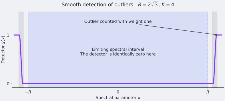
A smooth detector vanishes on a neighborhood of the limiting spectral interval and reaches one at the outlier threshold. The gray strip is a transition region; its width controls the derivative bounds in the probability estimate. The illustration uses the degree-four tree, with $R=2\sqrt{3}$ and $K=4$.

Distributions and their supports

A compactly supported distribution is a linear functional $\nu$ on smooth functions such that

$$|\nu (h)|\le C\sum _{j=0}^r\underset{|x|\le K}{\sup }|h^{(j)}(x)|$$

for some finite $C,r,K$. A measure is the order-zero case. Derivatives of point masses are also distributions:

$${\delta }_a(h)=h(a),{\delta }_a^{\prime }(h)=-h^{\prime }(a).$$

For example,

$$\begin{array}{rl}h(N^{-1})& =h(0)+N^{-1}{h}^{\prime }(0)\\ & +O_h(N^{-2})\end{array}$$

has correction ${\nu }_1=-{\delta }_0^{\prime }$. There is no reason to expect a general correction term to be a positive measure.

The support of $\nu$ is the smallest closed set $E$ such that $\nu (h)=0$ whenever $h$ vanishes on a neighborhood of $E$. Vanishing merely at the points of $E$ is insufficient for distributions: $h(0)=0$ need not imply ${\delta }_0^{\prime }(h)=0$.

Thus the detector argument needs two separate conclusions:

1. The polynomial trace expansion extends continuously to smooth functions.
2. The correction distribution satisfies $\mathrm{supp}{\nu }_1\subseteq [-R,R]$.

Rationality by itself does not imply the second conclusion. The diagonal outlier example has the exact rational expansion

$${\mathrm{tr}}_{N}h(X^N)=h(0)+\frac{h(2)-h(0)}{N},$$

so ${\nu }_1={\delta }_2-{\delta }_0$ has support outside the limiting spectrum.

flowchart TD
  A["Rational formulas for expected traces"] --> B["Markov inequality and interpolation"]
  B --> C["Polynomial remainder bounds"]
  C --> D["Chebyshev expansion and Fourier estimates"]
  D --> E["Smooth trace expansion"]
  F["Asymptotics of fixed words"] --> G["Growth bounds for correction moments"]
  G --> H["Support inside the limiting norm interval"]
  E --> I["Smooth detector excludes outliers"]
  H --> I
  J["Trace convergence in probability"] --> L["Lower norm bound"]
  I --> M["Strong convergence"]
  L --> M

🏷️ Rational trace formulas from permutation constraints

For a word $w$, the full permutation trace is its number of fixed points. Removing the constant vector gives

$${\mathrm{Tr}}_{H_N}w({\mathbf{S}}^N)=\#\mathrm{Fix}(w(\mathbf{\sigma }))-1.$$

To count fixed points, follow a labeled closed walk encoding the word. Identify positions that visit the same vertex. Each resulting quotient graph $\Gamma$ has $v_{\Gamma }$ vertices and $e_{\Gamma }^j$ distinct constraints of color $j$, meaning constraints imposed on the permutation ${\sigma }_j$.

A valid quotient must specify a partial bijection for each color: two equal inputs cannot have different outputs, and two different inputs cannot have the same output. If the quotient is valid, there are

$$(N{)}_{v_{\Gamma }}=N(N-1)\cdots (N-v_{\Gamma }+1)$$

injective vertex labelings. A uniform permutation realizes a specified partial bijection with $a$ distinct inputs with probability $1/(N{)}_a$. Independence over colors therefore gives the contribution

$$\frac{(N{)}_{v_{\Gamma }}}{{\prod }_{j=1}^d(N{)}_{e_{\Gamma }^j}}.$$

Put $e_{\Gamma }={\sum }_j{e}_{\Gamma }^j$ and $x=1/N$. After division by $N$, this becomes

$$x^{e_{\Gamma }-v_{\Gamma }+1}\frac{{\prod }_{\ell =1}^{v_{\Gamma }-1}(1-\ell x)}{{\prod }_{j=1}^d{\prod }_{\ell =1}^{e_{\Gamma }^j-1}(1-\ell x)}.$$

The exponent is nonnegative because the quotient is connected. The identity word can be treated directly; all other contributions have this finite rational form. This is the source of rationality, rather than an approximation valid only asymptotically (Linial & Puder, 2010).

A denominator that works for every word of a given length

For words of length at most $L$, define

$$\begin{array}{rl}{g}_L(x)& =\prod _{j=1}^{L-1}(1-jx{)}^{a_j},\\ a_j& =\min \left(d,\lfloor \frac{L}{j+1}\rfloor \right).\end{array}$$

The exponent $a_j$ bounds the number of colors that can each have at least $j+1$ distinct constraints. Consequently, for $N\ge L$,

$$\mathbb{E}{\mathrm{tr}}_{N}w({\mathbf{S}}^N)=\frac{f_w(1/N)}{g_L(1/N)},$$

with numerator and denominator degrees at most $L(1+\log d)$. The logarithm comes from summing the bound $\min (d,L/(j+1))$ over $j$. The graph formula also bounds the numerator degree after denominators are cleared; one does not need to compute its coefficients individually.

If $h$ has degree at most $q$, the words in $h(P)$ have length at most $q{q}_0$. Hence

$$\begin{array}{rl}\mathbb{E}{\mathrm{tr}}_{DN}h(X_N)& ={\Psi }_h(1/N),\\ {\Psi }_h(x)& =\frac{f_h(x)}{g_{q{q}_0}(x)}.\end{array}$$

The function is analytic near zero, and its Taylor coefficients define linear functionals

$${\nu }_j(h)=\frac{{\Psi }_h^{(j)}(0)}{j!}.$$

These coefficients do not depend on an artificially enlarged degree bound $q$: two rational descriptions agreeing at all sufficiently small reciprocal integers agree identically near zero.

The first coefficients and proper powers

A nonidentity element $v\in {\mathbb{F}}_d$ is a proper power if $v=u^k$ for some $k\ge 2$. Every nonidentity element can be written uniquely as $u^k$ with $k\ge 1$ and $u$ not itself a proper power. This is different from being primitive, which will arise later.

Let $\omega (k)$ be the number of positive divisors of $k$. For $w=u^k\ne e$ with $u$ not a proper power, Nica’s word asymptotics, recalled in §5 of the source, give

$$\underset{N\to \infty }{\lim }\mathbb{E}{\mathrm{Tr}}_{H_N}w=\omega (k)-1.$$

One can see the divisor count directly for $w=g_1^k$. A point is fixed by ${\sigma }_1^k$ exactly when its cycle length divides $k$. A uniform permutation has expected number $1/\ell$ of cycles of length $\ell \le N$, so

$$\mathbb{E}\#\mathrm{Fix}({\sigma }_1^k)=\#\{\ell :\ell \mid k,\ell \le N\}.$$

For $N\ge k$ this is $\omega (k)$. For general words, the quotient-graph count gives the same leading answer: after cyclic reduction, order-one contributions come from rank-one quotients, whose possible cyclic periods are the divisors of the power exponent. Higher-rank quotients have an additional negative power of $N$.

In particular, a non-power word has limiting restricted trace zero. This yields weak convergence to the free tuple and identifies the first correction: identity words contribute $-1$, non-power words contribute $0$, and proper powers contribute $\omega (k)-1$.

A normalization check

For the constant test function,

$$\begin{array}{c}{\nu }_0(1)=1,{\nu }_1(1)=-1,\\ {\nu }_j(1)=0(j\ge 2).\end{array}$$

Thus a Taylor remainder vanishes on constants once terms through order $N^{-1}$ have been retained. We use the smooth remainder estimate below with expansion order $m\ge 2$. At order $m=1$, a derivative-only remainder estimate would need an additional constant contribution because the trace is divided by $N$, not $N-1$.

🏷️ Markov interpolation and the polynomial master inequality

The rational function ${\Psi }_h$ has a spectral interpretation at $x=1/N$, but its derivatives require control between those points. The classical polynomial inequality of A. and V. Markov supplies that control.

Markov's derivative inequality

If $f$ is a real polynomial of degree at most $Q$ on $[0,a]$, then

$$\begin{array}{rl}& \Vert f^{(m)}{\Vert }_{\infty }\\ & \le \frac{1}{(2m-1)!!}{\left(\frac{2Q^2}{a}\right)}^m\Vert f{\Vert }_{\infty }.\end{array}$$

In particular, $\Vert f^{\prime }{\Vert }_{\infty }\le 2Q^2\Vert f{\Vert }_{\infty }/a$. Here $(2m-1)!!=1\cdot 3\cdots (2m-1)$.

This is an inequality about polynomial derivatives; it is distinct from the probabilistic Markov inequality used to bound the detector trace. The $Q^2$ scale is sharp, as the endpoint derivatives of Chebyshev polynomials show. Rescaling the standard inequality on $[-1,1]$ gives the factor $2/a$.

Recovering a uniform bound from a fine grid

Suppose every point of $[0,a]$ lies within distance $a/(4Q^2)$ of a sampling set $I$. At a maximum point $x_{\ast }$, choose a nearby sample $y$. The mean value theorem gives

$$\begin{array}{rl}|f(x_{\ast })|& \le |f(y)|+|x_{\ast }-y|\Vert f^{\prime }{\Vert }_{\infty }\\ & \le \underset{I}{\sup }|f|+\frac{1}{2}\Vert f{\Vert }_{\infty }.\end{array}$$

Therefore

$$\Vert f{\Vert }_{C^0[0,a]}\le 2\underset{I}{\sup }|f|.$$

For the reciprocal grid $I=\{0\}\cup \{1/N:N\ge M\}$, adjacent gaps are of size at most $M^{-2}$. Thus taking $M\ge 4Q^2$ is a convenient sufficient condition on the interval $[0,1/M]$. The paper tracks constants slightly more efficiently; the relevant scale is $M\asymp Q^2$.

The denominator is nearly constant

The product defining $g_L$ satisfies

$$\begin{array}{c}{e}^{-1}\le g_L(x)\le 1\\ \text{for }0\le x\le \frac{1}{L^2(1+\log d)}.\end{array}$$

Indeed, its total degree is at most $L(1+\log d)-1$, every factor is at least $1-Lx$, and

$$(1-1/u{)}^{u-1}\ge e^{-1}(u>1).$$

The empty product when $L=1$ is simply one. In particular, no pole lies in the short interval used for interpolation.

At a reciprocal integer in that interval, functional calculus gives

$$|{\Psi }_h(1/N)|\le \Vert h{\Vert }_{C^0[-K,K]}.$$

Set $Q=q{q}_0(1+\log d)$ and take $M\asymp Q^2$. Apply the grid estimate to $f_h=g_{q{q}_0}{\Psi }_h$, and then divide by the denominator bound. This yields

$$\Vert {\Psi }_h{\Vert }_{C^0[0,1/M]}\le 2e\Vert h{\Vert }_{C^0[-K,K]}.$$

Derivatives of a rational function

If $r=f/g$, both degrees are at most $Q$, and

$$c=\underset{x,y\in [0,a]}{\sup }\left|\frac{g(x)}{g(y)}\right|<\infty ,$$

then the rational version of Markov’s inequality is

$$\Vert r^{(m)}{\Vert }_{\infty }\le m!{\left(\frac{5c{Q}^2}{a}\right)}^m\Vert r{\Vert }_{\infty }.$$

To derive it, differentiate $f=rg$:

$$r^{(m)}g=f^{(m)}-\sum _{j=1}^m\left(\genfrac{}{}{0ex}{}{m}{j}\right)r^{(m-j)}{g}^{(j)}.$$

Apply polynomial Markov bounds to $f^{(m)}$ and $g^{(j)}$, divide by $g$, and induct on $m$. The combinatorial identity

$$\left(\genfrac{}{}{0ex}{}{m}{j}\right)\frac{(m-j)!}{(2j-1)!!}=\frac{2^{j}m!}{(2j)!}$$

controls the induction sum by a convergent hyperbolic-cosine series. Thus the denominator costs only a fixed factor per derivative when $c\le e$.

Here $a=1/M\asymp Q^{-2}$. Each derivative therefore costs $Q^4$: one $Q^2$ from Markov’s inequality and one $Q^2$ from shrinking the interpolation interval. Write the remainder and a constant as

$$\begin{array}{rl}{\mathcal{R}}_{m,N}(h)& =\mathbb{E}{\mathrm{tr}}_{DN}h(X_N)\\ & -\sum _{j=0}^{m-1}\frac{{\nu }_j(h)}{N^j},\\ C_0& =4q_0(1+\log d).\end{array}$$

Taylor’s theorem now gives the central estimate.

Polynomial master inequality

For every integer $m\ge 1$ and every real polynomial $h$ of degree at most $q\ge 1$,

$$\begin{array}{rl}& |{\mathcal{R}}_{m,N}(h)|\\ & \le \frac{(q{C}_0{)}^{4m}}{N^m}\Vert h{\Vert }_{C^0[-K,K]}.\end{array}$$

The displayed constant is the one in Theorem 6.1 of the paper.

Taylor’s theorem first proves the estimate when $N\ge M$. Taking $N\to \infty$ in successive remainders also gives

$$|{\nu }_j(h)|\le (4q{q}_0(1+\log d){)}^{4j}\Vert h{\Vert }_{\infty }.$$

For $N<M$, bound the expected trace and each Taylor coefficient separately. In this regime the right-hand side is already sufficiently large; the coefficient bounds close the estimate by a geometric-sum comparison. Thus the final statement holds for all $N$, not merely the reciprocal integers used to derive it.

Taking $m=2$ yields the $q^8/N^2$ remainder. It is important that this is multiplied by $\Vert h{\Vert }_{\infty }$, rather than by the sum of absolute values of the monomial coefficients of $h$.

🏷️ Chebyshev expansions and the passage to smooth functions

A direct approximation of a smooth function by degree-$q$ polynomials does not settle the extension problem: the remainder estimate grows like $q^{4m}$. Instead, resolve the test function into individual bounded polynomials and sum their errors.

The Chebyshev polynomial $T_j$ is defined by

$$T_j(\cos \theta )=\cos (j\theta ).$$

Thus $\Vert T_j{\Vert }_{C^0[-1,1]}=1$. For a polynomial $h$, write

$$\begin{array}{rl}h(x)& =\sum _{j=0}^q{a}_j{T}_j(x/K),\\ f(\theta )& =h(K\cos \theta )=\sum _{j=0}^q{a}_j\cos (j\theta ).\end{array}$$

The Chebyshev coefficients are Fourier cosine coefficients. Applying the master inequality separately to $T_j(x/K)$ replaces

$$q^{4m}\Vert h{\Vert }_{\infty }\text{by}\sum _{j\ge 1}{j}^{4m}|a_j|.$$

For $m\ge 2$, the constant term contributes no remainder, by the normalization check above.

Fourier decay as a derivative estimate

An elementary estimate already suffices for qualitative convergence. For any nonnegative integer $r$,

$$\begin{array}{rl}& \sum _{j\ge 1}{j}^r|a_j|\\ & \le \frac{\pi }{\sqrt{6}}{\left(\sum _{j\ge 1}{j}^{2r+2}|a_j{|}^2\right)}^{1/2}\\ & \lesssim \Vert f^{(r+1)}{\Vert }_{L^2[0,2\pi ]}.\end{array}$$

The first inequality is Cauchy–Schwarz, using ${\sum }_{j\ge 1}{j}^{-2}={\pi }^2/6$, and the second is Parseval’s identity. The chain rule then bounds this by $C_{r,K}\Vert h{\Vert }_{C^{r+1}[-K,K]}$.

For the sharper dependence on the detector width, the paper uses

$$\begin{array}{c}\sum _{j\ge 1}{j}^r|a_j|\lesssim {\beta }_{\ast }\Vert f^{(r+1)}{\Vert }_{L^{\beta }[0,2\pi ]},\\ {\beta }_{\ast }=\frac{\beta }{\beta -1},\beta >1.\end{array}$$

This is a classical Fourier estimate associated with Zygmund. Its relevant mechanism is particularly transparent for $1<\beta \le 2$. Hausdorff–Young bounds the ${\ell }^{{\beta }_{\ast }}$ norm of the Fourier coefficients of $f^{(r+1)}$ by its $L^{\beta }$ norm. Hölder’s inequality, applied with weights $1/j$, then bounds the sum by

$$\begin{array}{rl}& {\left(\sum _{j\ge 1}{j}^{-\beta }\right)}^{1/\beta }\Vert f^{(r+1)}{\Vert }_{L^{\beta }}\\ & \lesssim {\beta }_{\ast }\Vert f^{(r+1)}{\Vert }_{L^{\beta }}.\end{array}$$

For $\beta \ge 2$, the preceding $L^2$ argument and the finite measure of the circle suffice.

Extension of the coefficient functionals

Suppose a functional on polynomials satisfies

$$|\nu (h)|\le C{q}^r\Vert h{\Vert }_{C^0[-K,K]}.$$

Its value on $T_j(x/K)$ grows at most polynomially in $j$. The Fourier estimate gives

$$|\nu (h)|\le C^{\prime }\Vert h{\Vert }_{C^{r+1}[-K,K]}.$$

The constant Chebyshev coefficient is bounded separately by $|\nu (1)|\Vert h{\Vert }_{\infty }$. Polynomial approximation in the $C^{r+1}$ norm now gives a unique continuous extension. To justify this density, approximate the highest derivative uniformly by a polynomial, integrate repeatedly, and match the lower derivatives at one endpoint.

The extension is a compactly supported distribution. Applying the same argument to the remainder proves the smooth master inequality:

$$\begin{array}{rl}& |{\mathcal{R}}_{m,N}(h)|\\ & \lesssim \frac{C_0^{4m}}{N^m}{\beta }_{\ast }\Vert f^{(4m+1)}{\Vert }_{L^{\beta }},m\ge 2.\end{array}$$

This establishes that ${\nu }_1(h)$ is meaningful for smooth $h$. Formal substitution into a moment expansion would not have justified that conclusion.

The Chebyshev scaling uses the deterministic bound $K$, not the limiting edge $R$. Here these polynomials serve as a bounded Fourier basis; the argument does not use their separate interpretation through nonbacktracking walks.

🏷️ Bounding distributional support by moments

Support from exponential moment growth

If $\nu$ is a compactly supported distribution and

$$\rho =\underset{p\to \infty }{\mathrm{limsup}}|\nu (x^p){|}^{1/p},$$

then $\mathrm{supp}\nu \subseteq [-\rho ,\rho ]$.

For positive measures, even moments make this intuitive: mass beyond $\rho +\eta$ would force faster exponential growth. Distributions may have signs and derivatives, so a proof using positivity is unavailable.

Proof: Cauchy transform and distributional support

Use the Cauchy transform

$$\begin{array}{c}F(z)=\nu \left(x\mapsto \frac{1}{z-x}\right),\\ \mathrm{Im}z\ne 0.\end{array}$$

Outside a disk containing the support, the geometric series converges together with sufficiently many derivatives in $x$. Therefore

$$F(z)=\sum _{p=0}^{\infty }\frac{\nu (x^p)}{z^{p+1}}.$$

The root test makes the series analytic throughout $|z|>\rho$. To relate this to support, observe in the distributional sense that

$$\begin{array}{rl}& \frac{F(t-i\eta )-F(t+i\eta )}{2\pi i}\\ & ={\nu }_x\left(\frac{\eta }{\pi ((t-x{)}^2+{\eta }^2)}\right).\end{array}$$

The right side is convolution with the Poisson kernel and tends to $\nu$ as $\eta \downarrow 0$. If the Cauchy transform extends holomorphically across a real interval, the jump on the left tends to zero there. The distribution therefore vanishes on that interval. The Laurent series provides exactly such an extension outside $[-\rho ,\rho ]$.

Consequently, a bound

$$|{\nu }_1(x^p)|\le C(p+1{)}^a{R}^p$$

is enough to locate the support inside $[-R,R]$: polynomial factors disappear after taking $p$th roots. The order of limits is crucial. First take $N\to \infty$ to extract ${\nu }_1(x^p)$ for fixed $p$; then let $p\to \infty$. No estimate on matrix moments at $p\gg \log N$ is needed.

🏷️ The support calculation for random regular graphs

Expand $A_N^p$ as a sum of words of length $p$ in the $2d$ generators and inverses. Let $c_p(v)$ be the number of these words that reduce to $v\in {\mathbb{F}}_d$. Equivalently,

$$c_p(v)=⟨{\delta }_v,A_F^p{\delta }_e⟩.$$

The identity-word contribution and the proper-power asymptotics give

$$\begin{array}{rl}& {\nu }_1(x^p)=-\tau (A_F^p)\\ & +\sum _{k=2}^p(\omega (k)-1)\sum _{v\in {\mathbb{F}}_d^{\mathrm{np}}}{c}_p(v^k),\end{array}$$

where ${\mathbb{F}}_d^{\mathrm{np}}$ denotes the nonidentity elements that are not proper powers.

The main combinatorial estimate is

$$\begin{array}{c}\sum _{v\in {\mathbb{F}}_d^{\mathrm{np}}}{c}_p(v^k)\le (p+1{)}^4{R}^p,\\ k\ge 2,\end{array}$$

with $R=\Vert A_F\Vert$. Here is the mechanism behind it.

Cyclic reduction and a five-piece decomposition

A reduced word is cyclically reduced if its last letter is not the inverse of its first. Every nonidentity reduced word has a unique decomposition

$$v=gu{g}^{-1},$$

where $u$ is cyclically reduced and the displayed concatenation is reduced. It follows that

$$v^k=g{u}^k{g}^{-1}=guu{u}^{k-2}{g}^{-1}.$$

Because the Cayley graph is a tree, a walk ending at this vertex must visit the intermediate vertices along the unique geodesic. Thus its word can be split at four times

$$0\le t_1\le t_2\le t_3\le t_4\le p$$

into pieces reducing to $g,u,u,u^{k-2},g^{-1}$. Empty pieces handle $g=e$ or $k=2$.

There may be several possible splitting times. For the adjacency polynomial every coefficient is nonnegative, so counting all choices gives a valid upper bound. This positivity is a special feature of the present argument.

For fixed times, the contribution becomes a sum of products

$$\begin{array}{rl}& c_{t_1}(g)c_{t_2-t_1}(u)c_{t_3-t_2}(u)\\ & \times c_{t_4-t_3}(u^{k-2})c_{p-t_4}(g^{-1}).\end{array}$$

Bound the middle factor by $R^{t_4-t_3}$. For the pair indexed by $u$, use

$$\begin{array}{rl}& \sum _u|c_a(u)c_b(u)|\\ & \le {\left(\sum _u|c_a(u){|}^2\sum _v|c_b(v){|}^2\right)}^{1/2}\\ & =\Vert A_F^a{\delta }_e{\Vert }_2\Vert A_F^b{\delta }_e{\Vert }_2\\ & \le R^{a+b}.\end{array}$$

The same inequality applies to the pair indexed by $g$, because inversion permutes the group elements. The five exponents add to $p$, so each choice of times contributes at most $R^p$. There are at most $(p+1{)}^4$ choices.

Finally, $\omega (k)-1\le k\le p$, so

$$|{\nu }_1(x^p)|\le (1+p^2(p+1{)}^4)R^p.$$

The support theorem yields

$$\mathrm{supp}{\nu }_1\subseteq [-R,R].$$

This completes the only model-specific support argument needed for the effective Friedman theorem (Chen et al., 2026, sec.8.1).

🏷️ The detector width and the eighth power

The preceding arguments already imply a qualitative upper bound. To recover the stated probability estimate, one must keep track of how the smooth detector depends on $\epsilon$.

An ordinary $C^9$ bound would cost roughly ${\epsilon }^{-9}$. The improvement to an eighth power with a logarithm comes from estimating the ninth derivative in $L^{\beta }$ with $\beta$ close to one.

Constructing the cutoff in angular coordinates

Let $F\ge 0$ be a smooth probability density supported in $[0,1]$, and set

$$\begin{array}{rl}{F}_a(x)& =a^{-1}F(x/a),\\ H_a(x)& =a^{-1}{1}_{[0,a]}(x).\end{array}$$

For an integer $r\ge 1$, define a smooth increasing function $u$ by

$$\begin{array}{c}{u}^{\prime }(x)=F_{\delta /2}\ast H_{\delta /(2r)}^{\ast r},\\ u(-\infty )=0.\end{array}$$

Here $\ast$ denotes convolution, $(f\ast g)(x)=\int f(x-y)g(y)dy$, and $H_a^{\ast r}$ is the convolution of $r$ copies of $H_a$. Then $u=0$ on $(-\infty ,0]$ and $u=1$ on $[\delta ,\infty )$. Since

$$H_a^{\prime }=a^{-1}({\delta }_0-{\delta }_a),$$

its derivative has total variation $2/a$. Young’s convolution inequality therefore gives

$$\Vert u^{(r+1)}{\Vert }_{L^{\beta }}\le (Cr{)}^r{\delta }^{-r-1/{\beta }_{\ast }}.$$

Choose

$$\begin{array}{rl}\phi & =\arcsin \left(\frac{R+\epsilon /2}{K}\right),\\ \delta & =\arcsin \left(\frac{R+\epsilon }{K}\right)-\phi .\end{array}$$

On $[-K,K]$, put

$$\begin{array}{rl}\chi (x)& =u(\arcsin (x/K)-\phi )\\ & +u(-\arcsin (x/K)-\phi ),\end{array}$$

and extend it by one outside. The two transitions do not overlap, and $\chi$ is constant near $\pm K$, so the extension is smooth. It has exactly the required detector properties.

For $f(\theta )=\chi (K\cos \theta )$, the arcsine turns the transition into a translate of $u$ on each half-circle. Moreover, $\delta \ge \epsilon /(2K)$. Hence

$$\Vert f^{(r+1)}{\Vert }_{L^{\beta }}\le (Cr{)}^r{\left(\frac{K}{\epsilon }\right)}^{r+1/{\beta }_{\ast }}.$$

Taking $r=8$ and $m=2$ in the smooth master inequality, and using ${\nu }_0(\chi )={\nu }_1(\chi )=0$, gives

$$\begin{array}{rl}& \mathbb{P}\{\Vert X_N\Vert \ge R+\epsilon \}\\ & \lesssim \frac{D}{N}(q_0\log d{)}^8{\beta }_{\ast }{\left(\frac{K}{\epsilon }\right)}^{8+1/{\beta }_{\ast }}.\end{array}$$

Set $L=K/\epsilon >1$ and choose ${\beta }_{\ast }=1+\log L$. Then

$$L^{1/{\beta }_{\ast }}=\exp \left(\frac{\log L}{1+\log L}\right)\le e,$$

while ${\beta }_{\ast }=\log (eL)$. This proves the eighth power and logarithm in the main estimate, once first-order support is known. The factors have distinct origins: $N^{-2}$ comes from Taylor expansion, $DN$ counts possible eigenvalues, $q_0^8(\log d{)}^8$ comes from rational interpolation, and the detector supplies $(K/\epsilon {)}^8\log (eK/\epsilon )$.

🏷️ General polynomials and exact counting

For a general polynomial, the coefficients in a word expansion may be negative or complex, and matrix multiplication introduces additional cancellations. The preceding overcounting argument cannot be transferred by taking absolute values of every coefficient: that would replace the reduced norm $R$ by a potentially much larger coefficient bound.

The paper resolves this in two parts: a factorization with controlled operator norms, and an exact decomposition of paths.

Pisier’s factorization input

Fix $\eta >0$. A factorization theorem of Pisier supplies rectangular matrix-valued linear polynomials

$$\begin{array}{rl}{X}_j& =\sum _{i=0}^{2d}{B}_{j,i}\otimes \lambda (g_i),\\ X_F& =X_1{X}_2\cdots X_{\ell },\\ \Vert X_j\Vert & \le (R+\eta {)}^{1/\ell }.\end{array}$$

Here $g_0=e$, $g_{d+i}=g_i^{-1}$, and $B_{j,i}$ has size $D_j\times D_{j+1}$, with $D_1=D_{\ell +1}=D$. The length $\ell$ and intermediate dimensions may depend on $P$ and $\eta$ (Pisier, 2018). This is a genuine external input; factoring a polynomial into linear pieces algebraically would not by itself control their norms.

Equality in the free regular representation is equality of the reduced-word coefficients. It therefore remains valid after substituting any unitary tuple, including ${\mathbf{S}}^N$. Extend the factors periodically, so that $X_F^p=X_1\cdots X_{p\ell }$.

For fixed $\eta$, all intermediate dimensions are fixed as $p\to \infty$. This will allow them to disappear from exponential growth rates, even though they need not be small.

A first-visit identity

For a word of length $k$ and a nonidentity target $v$, write

$$g_{i_1}\cdots g_{i_k}\triangleq v$$

when its product is $v$ and no nonempty proper suffix has product $v$. Operators act on ${\delta }_e$ from right to left, so this says that the associated walk first reaches $v$ at its last step.

Let

$$Q=I-|{\delta }_e⟩⟨{\delta }_e|,L_j=\lambda (g_{i_j}).$$

Define

$$\begin{array}{rl}C(v)& =⟨{\delta }_v,L_1\cdots L_k{\delta }_e⟩,\\ B_s& =⟨{\delta }_e,L_{1}Q{L}_{2}Q\cdots Q{L}_s{\delta }_e⟩,\\ C_s(v)& =⟨{\delta }_v,L_{s+1}\cdots L_k{\delta }_e⟩.\end{array}$$

Then the exact identity is

$$1_{\{g_{i_1}\cdots g_{i_k}\triangleq v\}}=C(v)-\sum _{s=1}^{k-1}{B}_s{C}_s(v).$$

For $s=1$, there is no $Q$ in $B_s$. Each $Q$ excludes an intermediate return to the identity. The subtracted term indexed by $s$ identifies the last earlier visit to $v$, followed by a final excursion that returns to $v$ with no intervening visit. These alternatives are disjoint, so the identity preserves signed coefficients.

For example, $g_1{g}_2{g}_2^{-1}{g}_1=g_1^2$ admits several ordinary cuts into two pieces equal to $g_1$. Requiring the right-hand piece to be a first-visit word selects a unique cut.

Unique cuts at the reduced-word boundaries

Suppose $v_1\cdots v_a$ is a reduced concatenation of nonidentity group elements. Every word whose product is this concatenation has a unique split

$$\begin{array}{c}w=w_1{w}_2\cdots w_a,\\ w_1=v_1,w_j\triangleq v_j(j\ge 2).\end{array}$$

The cuts are determined successively by the first visits, read from the right, to the corresponding geodesic vertices. Substituting the preceding identity for each first-visit condition yields an exact sum of products of ordinary operator segments and segments with $Q$ inserted between factors.

Both types of segment obey the same norm estimate, because $\Vert Q\Vert =1$:

$$\begin{array}{rl}& \Vert X_t\cdots X_s\Vert \\ & \le (R+\eta {)}^{(s-t+1)/\ell },\\ & \Vert X_t(I\otimes Q)\cdots (I\otimes Q)X_s\Vert \\ & \le (R+\eta {)}^{(s-t+1)/\ell }.\end{array}$$

Now apply the exact decomposition to $v^k=guu{g}^{-1}$ when $k=2$, or to $guu{u}^{k-2}{g}^{-1}$ in general, omitting empty pieces. As in the adjacency argument, pair the two $u$ terms and the two $g$ terms by Cauchy–Schwarz.

There are at most five nonempty pieces, hence at most eight time indices after expanding the first-visit conditions, and at most nine intermediate matrix indices. Writing $D_{\max }={\max }_j{D}_j$, the resulting bound from Lemma 9.6 is

$$\begin{array}{rl}& \left|\sum _{v\in {\mathbb{F}}_d^{\mathrm{np}}}\sum _{i_1,\dots ,i_{p\ell }}{a}_{i_1,\dots ,i_{p\ell }}{1}_{\{g_{i_1}\cdots g_{i_{p\ell }}=v^k\}}\right|\\ & \le 2D_{\max }^9(p\ell {)}^8(R+\eta {)}^p,\end{array}$$

where

$$a_{i_1,\dots ,i_{p\ell }}={\mathrm{tr}}_D(B_{1,i_1}\cdots B_{p\ell ,i_{p\ell }}).$$

The two in the bound accounts for cyclically reduced roots and roots with a nonempty conjugating word. Summing over the power exponent gives

$$\begin{array}{rl}& |{\nu }_1(x^p)|\\ & \le R^p+2D_{\max }^9(p\ell {)}^{10}(R+\eta {)}^p.\end{array}$$

Take $p$th roots with $\eta$ fixed, then let $p\to \infty$, and only afterward let $\eta \downarrow 0$. The support theorem gives

$$\mathrm{supp}{\nu }_1\subseteq [-R,R].$$

The detector estimate now proves strong-convergence upper bounds for every fixed matrix polynomial. Exact counting is what allows the final exponential scale to remain $R$ despite signed coefficients (Chen et al., 2026, sec.9).

🏷️ Higher corrections and the staircase of rare events

For adjacency matrices, additional group-theoretic information locates the supports of higher correction distributions. Put $b=2d-1$ and $t_m=2m-1$, and define

$${\rho }_m=\{\begin{array}{ll}2\sqrt{b},& t_m\le \sqrt{b},\\ t_m+\frac{b}{t_m},& t_m>\sqrt{b},\end{array}$$

and

$$m_{\ast }=\lfloor \frac{\sqrt{2d-1}+1}{2}\rfloor .$$

Thus ${\rho }_1,\dots ,{\rho }_{m_{\ast }}$ all equal the tree edge, and subsequent thresholds increase up to ${\rho }_d=2d$.

Staircase theorem

Fix $d\ge 2$ and $m_{\ast }\le m\le d-1$. For

$$0<\epsilon <{\rho }_{m+1}-{\rho }_m,$$

the permutation model satisfies

$$\begin{array}{rl}& \mathbb{P}\{\Vert A_N\Vert \ge {\rho }_m+\epsilon \}\\ & \le \frac{C_d}{N^m{\epsilon }^{4(m+1)}}\log \left(\frac{2e}{\epsilon }\right),\\ & \mathbb{P}\{\Vert A_N\Vert \ge {\rho }_m+\epsilon \}\\ & \ge \frac{1-o(1)}{N^m}.\end{array}$$

The upper bound holds for every $N$; the lower bound is asymptotic with $d,m,\epsilon$ fixed (Chen et al., 2026, sec.3.2).

Thus a threshold strictly between ${\rho }_m$ and ${\rho }_{m+1}$ has tail probability of order $N^{-m}$. The theorem does not specify the behavior exactly at a transition point or uniformly as the threshold approaches one with $N$.

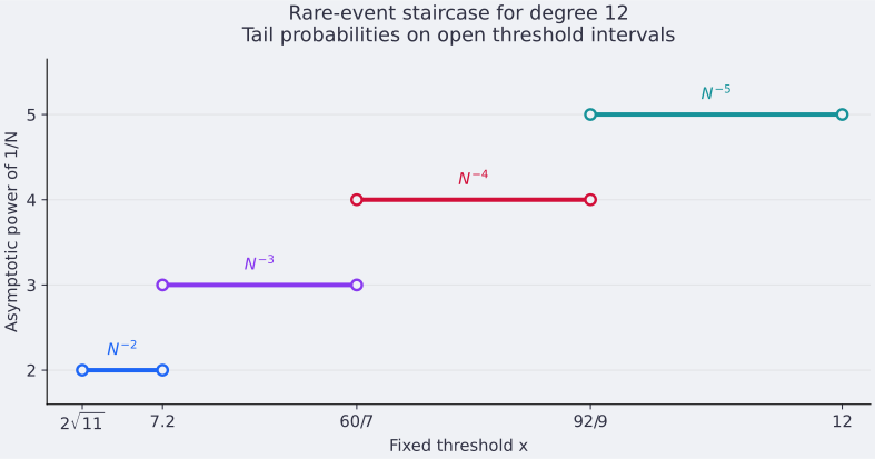
For $d=6$, the graph degree is $12$ and $m_{\ast }=2$. On each open interval the plot shows the limiting exponent $-\log \mathbb{P}\{\Vert A_N\Vert \ge x\}/\log N$. This is a plot of the theorem’s asymptotic exponents, not simulated probabilities. Open endpoints deliberately leave the transition values unspecified.

The higher-order word input

An element of a free group is primitive if it belongs to some free basis. For a word $w$, its primitivity rank $\pi (w)$ is the smallest rank of a subgroup containing $w$ in which $w$ is not primitive. Set $\pi (w)=\infty$ if no such subgroup exists, and $\pi (e)=0$. Proper powers have primitivity rank one. A word may be a non-power without being primitive; the commutator $g_1{g}_2{g}_1^{-1}{g}_2^{-1}$ is a basic example.

For finite positive primitivity rank, $\mathrm{Crit}(w)$ is the finite collection of subgroups attaining that minimum. Puder’s results control both the expansion coefficients of a word trace and the growth of the number of words with a given primitivity rank (Puder, 2015). In the form used by the source, for a nonidentity word,

$$\mathbb{E}{\mathrm{Tr}}_{H_N}w({\mathbf{S}}^N)=\sum _{s\ge 0}\frac{b_s(w)}{N^s},$$

and, writing $\pi =\pi (w)<\infty$,

$$\begin{array}{rl}{b}_s(w)& =0(s\le \pi -2),\\ b_{\pi -1}(w)& =|\mathrm{Crit}(w)|,\\ |b_s(w)|& \le |w{|}^{2(s+1)}(s\ge \pi ).\end{array}$$

Words with infinite primitivity rank have zero restricted expected trace. Let ${\mathcal{W}}_p^r$ be the set of length-$p$ letter sequences whose reduced product has primitivity rank $r$; different sequences with the same product are counted separately. The required counting theorem implies

$$\underset{p\to \infty }{\mathrm{limsup}}{\left(\sum _{w\in {\mathcal{W}}_p^r}|\mathrm{Crit}(w)|\right)}^{1/p}\le {\rho }_r.$$

These are the substantial external inputs for the staircase upper bound. Their role is precise: for $2\le m\le d$, only ranks at most $m$ can contribute to ${\nu }_m$, and

$$\begin{array}{rl}& |{\nu }_m(x^p)|\\ & \le m{p}^{2m}\underset{1\le r\le m}{\max }\sum _{w\in {\mathcal{W}}_p^r}|\mathrm{Crit}(w)|.\end{array}$$

The polynomial prefactor does not affect exponential growth. Since ${\rho }_r\le {\rho }_m$ for $r\le m$, the distributional support theorem gives

$$\mathrm{supp}{\nu }_m\subseteq [-{\rho }_m,{\rho }_m].$$

For a detector starting just beyond ${\rho }_m$, all terms ${\nu }_0,\dots ,{\nu }_m$ vanish. The smooth expansion now leaves a normalized remainder of order $N^{-(m+1)}$. Multiplying by $N$ yields the probability scale $N^{-m}$; the same cutoff calculation, with derivative order $4(m+1)+1$, gives the displayed dependence on $\epsilon$.

Loops explain the matching lower bound

The threshold formula itself has a concrete spectral interpretation. Consider an infinite graph with $k$ loops at a root, $r-2k$ ordinary branches leaving the root, and $r$-regular tree structure thereafter. Each loop contributes two at the root.

Try a radial eigenfunction with value $a^j$ at distance $j$. Away from the root and at the root, respectively, the eigenvalue equations are

$$\begin{array}{rl}\lambda & =a^{-1}+(r-1)a,\\ \lambda & =2k+(r-2k)a.\end{array}$$

Equating them gives

$$(2k-1)a^2-2ka+1=0.$$

Besides $a=1$, the decaying root is $a=(2k-1{)}^{-1}$. It defines an ${\ell }^2$ eigenfunction when

$$\begin{array}{c}(r-1)a^2<1\\ ⟺2k-1>\sqrt{r-1}.\end{array}$$

The eigenvalue is then

$$\lambda =(2k-1)+\frac{r-1}{2k-1}={\rho }_k.$$

At equality the candidate is not square summable; below the threshold it does not create this localized eigenvalue beyond the tree edge. When $k=d$, all branches disappear and the root is an isolated vertex with adjacency eigenvalue $2d$.

Now fix $k\ge 2$ specified permutation colors. Let $Z$ count vertices fixed by all $k$ permutations. Exact independence and uniformity give

$$\begin{array}{rl}\mathbb{E}Z& =N^{1-k},\\ \mathbb{E}[Z(Z-1)]& =(N(N-1){)}^{1-k}.\end{array}$$

The first moment and the first two terms of inclusion–exclusion imply

$$\mathbb{P}\{Z\ge 1\}=(1+o(1))N^{1-k}.$$

Conditional on the specified loops, a fixed-radius neighborhood outside them is a tree with probability tending to one. Truncate the preceding localized eigenfunction at a sufficiently large fixed radius. Its Rayleigh quotient can be made arbitrarily close to ${\rho }_k$ from below. Projecting off the constant vector changes this fixed-support test by a quantity tending to zero as $N\to \infty$. Thus it also detects an eigenvalue of $A_N$.

Choosing $k=m+1$ proves the lower bound for every fixed threshold below ${\rho }_{m+1}$. This also explains why an $O(N^{-1})$ upper tail is optimal in general: for $2\le d\le 4$, we have $m_{\ast }=1$.

Dependence on the graph model

The staircase includes loop configurations and belongs to the permutation model. High-probability convergence statements can be transferred to standard fixed-degree regular graph models by suitable comparison results, but those results do not preserve exact probabilities of order $N^{-m}$. In particular, a simple graph cannot contain the loop events used in this lower bound.

The source also proves $\Vert A_N\Vert =(1+o(1))2\sqrt{2d-1}$ when $d=d(N)$ varies arbitrarily with $N$, within the permutation model. Its proof combines the displayed effective Friedman bound in the range $d\le (\log N{)}^5$ with a separate existing high-degree estimate for the complementary range. The arbitrary-degree statement is therefore not obtained by substituting all possible $d(N)$ into the eighth-power bound alone.

🏷️ Stable representations and larger random matrices

A finite-dimensional unitary representation of the symmetric group is a homomorphism

$${\pi }_N:{\mathfrak{S}}_N⟶U(V_N).$$

Its character is ${\chi }_{{\pi }_N}(\sigma )=\mathrm{Tr}{\pi }_N(\sigma )$. Characters are constant on conjugacy classes. A representation is irreducible when it has no proper nonzero invariant subspace, and the trivial representation is the one-dimensional action fixing every vector.

Define the fixed-point statistics

$${\xi }_j(\sigma )=\#\mathrm{Fix}({\sigma }^j).$$

If $C_{\ell }(\sigma )$ counts cycles of length $\ell$, then

$${\xi }_j(\sigma )=\sum _{\ell \mid j}\ell C_{\ell }(\sigma ).$$

Thus these statistics encode cycle structure. A sequence $({\pi }_N{)}_{N\ge N_0}$ is stable, in the sense used here, if there is one fixed polynomial $\phi$ such that

$${\chi }_{{\pi }_N}(\sigma )=\phi ({\xi }_1(\sigma ),\dots ,{\xi }_r(\sigma ))$$

for every $N\ge N_0$. The same polynomial must work at all those dimensions.

Examples and dimensions

The standard representation on $H_N$ has $\phi ={\xi }_1-1$. A second example is its exterior square, whose character is

$$\frac{({\xi }_1-1{)}^2-({\xi }_2-1)}{2}$$

and whose dimension is $(N-1)(N-2)/2$. The identity follows from

$$\mathrm{Tr}({\wedge }^{2}T)=\frac{(\mathrm{Tr}T{)}^2-\mathrm{Tr}(T^2)}{2}.$$

Irreducible examples are indexed by a fixed partition $\lambda =({\lambda }_1\ge \cdots \ge {\lambda }_a>0)$. For $N\ge |\lambda |+{\lambda }_1$, attach a long first row:

$$\lambda [N]=(N-|\lambda |,{\lambda }_1,\dots ,{\lambda }_a).$$

The corresponding irreducible characters are stable. Every stable representation considered in the paper is a finite direct sum of such fixed families, with fixed multiplicities.

Assume that the representation is nonzero and has no trivial constituent. Its dimension is

$$D_N={\chi }_{{\pi }_N}(e)=\phi (N,\dots ,N),$$

so $D_N$ is a polynomial in $N$. Write $\alpha =\mathrm{deg}{D}_N$, giving $D_N\asymp N^{\alpha }$. The random matrices are

$${\Pi }_i^N={\pi }_N({\sigma }_i).$$

The coefficient dimension $D$ of $P$ and the representation dimension $D_N$ are different quantities. The total matrix dimension is $D{D}_N$. Write

$$Z_N=P({\mathbf{\Pi }}^N,{\mathbf{\Pi }}^{N\ast }).$$

Strong convergence for a fixed stable representation

Under the preceding assumptions, for a self-adjoint polynomial $P$ of degree $q_0\ge 1$,

$$\begin{array}{rl}& \mathbb{P}\{\Vert Z_N\Vert \ge R+\epsilon \}\\ & \le \frac{CD}{N}{\left(\frac{K{q}_0\log d}{\epsilon }\right)}^{4(\alpha +1)}\\ & \cdot \log \left(\frac{eK}{\epsilon }\right).\end{array}$$

Here $0<\epsilon <K-R$, $N\ge N_0$, and $C$ depends on the fixed stable family (Chen et al., 2026, sec.3.4).

In particular, the one-sided rate is $O_{\mathbb{P}}((\log N/N{)}^{1/(4(\alpha +1))})$. A representation with a trivial constituent would retain the scalar evaluation $P(1,\dots ,1)$ and can violate the conclusion.

The word-measure inputs

Set

$$b_{\phi }=\mathrm{deg}\phi (x_1,x_2^2,\dots ,x_r^r).$$

This weighted degree bounds the total length of permutation constraints needed to expand a character monomial. For a nonidentity word $w$ of length $L$, the expected unnormalized trace is rational in $1/N$, with denominator of the same form as before but with $L$ replaced by $b_{\phi }L$.

The relevant lowest-order asymptotics are

$$\underset{N\to \infty }{\lim }\mathbb{E}\mathrm{Tr}{\pi }_N(u(\mathbf{\sigma }{)}^k)=\varpi (k),$$

for any non-power $u$, where

$$\varpi (1)=0,|\varpi (k)|\le C_{\phi }{k}^{b_{\phi }}.$$

These facts follow from the word-measure results of Hanany and Puder (Hanany & Puder, 2023), as specialized in §10.1 of the source. They replace the divisor count $\omega (k)-1$ in the standard representation.

The polynomial growth has a useful cycle-count explanation. In the limit for a non-power word, finite collections of cycle counts behave like independent Poisson variables $Z_{\ell }$ with means $1/\ell$. Put $Y_j={\sum }_{\ell \mid j}\ell Z_{\ell }$. Then $\varpi (k)$ is obtained by evaluating the character polynomial on $(Y_k,Y_{2k},\dots ,Y_{rk})$ and taking expectation.

For a character monomial ${\xi }_1^{a_1}\cdots {\xi }_r^{a_r}$, form a multiset $S$ containing $jk$ with multiplicity $a_j$. The joint-moment formula is

$$\sum _{\mathcal{P}\in \mathrm{Partitions}(S)}\prod _{B\in \mathcal{P}}\left(\sum _{\ell \mid \gcd (B)}{\ell }^{|B|-1}\right).$$

Occurrences in the multiset are distinguished when forming partitions. Each block factor is at most $(rk{)}^{|B|}$, and the number of occurrences is at most $b_{\phi }$. This yields the claimed power bound. At $k=1$, the expectation of a nontrivial character under uniform permutations is zero; the absence of a trivial constituent is reflected in $\varpi (1)=0$.

Why expansion through order $\alpha$ is enough

It is convenient to normalize by $N^{\alpha }$, rather than by $D{D}_N$. For a fixed polynomial $h$, separate identity words from nonidentity words to get

$$\begin{array}{rl}& N^{-\alpha }\mathbb{E}\mathrm{Tr}h(Z_N)\\ & =\frac{D_N}{N^{\alpha }}({\mathrm{Tr}}_D\otimes \tau )(h(X_F))\\ & +O_h(N^{-\alpha }).\end{array}$$

The prefactor $D_N/N^{\alpha }$ is a polynomial in $1/N$ of degree at most $\alpha$. Thus the correction distributions of orders $0,\dots ,\alpha -1$ are scalar multiples of the free spectral distribution. Their supports already lie in $[-R,R]$.

At order $\alpha$, the only new contribution comes from the limits $\varpi (k)$ of nonidentity word traces. Because $\varpi (1)=0$, only proper powers remain. The same exact first-visit decomposition bounds the corresponding moments by

$$C_{P,\eta }(p\ell {)}^{9+b_{\phi }}(R+\eta {)}^p.$$

Taking $p$th roots and then $\eta \downarrow 0$ shows that this last required distribution also has support in $[-R,R]$.

Rational interpolation and Fourier expansion now give a smooth remainder of order $N^{-(\alpha +1)}$ after retaining orders $0$ through $\alpha$. A detector kills all those terms. Undoing the normalization multiplies by $N^{\alpha }$, leaving probability order $N^{-1}$. The interpolation cost is ${\epsilon }^{-4(\alpha +1)}$, explaining the exponent in the theorem.

Schreier graphs on tuples

Fix $k$. Let the symmetric group act on the ordered $k$-tuples of distinct elements of $\{1,\dots ,N\}$. This action is transitive and has $(N{)}_k$ states. Its permutation character is

$$({\xi }_1{)}_k={\xi }_1({\xi }_1-1)\cdots ({\xi }_1-k+1),$$

because a tuple is fixed exactly when all its entries are fixed. Removing constants gives the stable character $({\xi }_1{)}_k-1$ and dimension $(N{)}_k-1$.

Choose $d$ random permutations and join every tuple to its images under those permutations and their inverses. The resulting random Schreier graph has degree $2d$. The stable-representation theorem gives

$$\Vert \sum _{i=1}^d({\Pi }_i^N+{\Pi }_i^{N\ast })\Vert \stackrel{\mathbb{P}}{\to }2\sqrt{2d-1}.$$

Thus the same $d$ permutations generate near-optimal spectral behavior on a state space of size comparable to $N^k$, for every fixed $k$.

The constants in this theorem depend on the stable family. Allowing that family, or $k$, to grow with $N$ requires additional uniform estimates. Likewise, this fixed-family result does not prove expansion simultaneously across all irreducible representations, as would be needed for the full random Cayley graph of ${\mathfrak{S}}_N$.

🏷️ The lower bound and convergence in probability

An upper bound on outliers alone does not establish norm convergence. The lower bound uses the limiting trace’s faithfulness, but first requires convergence of traces in probability. Expected trace convergence by itself is insufficient.

We give the argument for stable representations, which includes standard permutation matrices. It is enough to work with one irreducible stable family and scalar polynomial coefficients: a fixed finite direct sum and the diagonal entries of a fixed coefficient matrix reduce the general trace statement to these cases.

Let $M=P({\mathbf{\Pi }}^N,{\mathbf{\Pi }}^{N\ast })$ be self-adjoint and introduce an independent uniform permutation ${\sigma }_0$, with $U={\pi }_N({\sigma }_0)$. Schur’s lemma gives the averaging identity

$${\mathbb{E}}_U[UM{U}^{\ast }]={\mathrm{tr}}_{D_N}(M)I.$$

Indeed, the average commutes with the irreducible representation, so it is scalar; taking its trace determines the scalar. Consequently,

$$\mathbb{E}{\mathrm{tr}}_{D_N}(UM{U}^{\ast }M)=\mathbb{E}({\mathrm{tr}}_{D_N}M{)}^2.$$

The left side is the expected trace of another fixed polynomial, now in $d+1$ independent permutations. Its free limit is

$$\tau (s_{0}P(\mathbf{s})s_0^{\ast }P(\mathbf{s}))=\tau (P(\mathbf{s}){)}^2,$$

where $s_0$ is a new free generator. To verify the identity, expand both copies of $P$ into words in the original generators. The product $g_{0}u{g}_0^{-1}v$ reduces to the identity only when both $u$ and $v$ are the identity. Thus the limiting second moment equals the square of the limiting first moment:

$$\mathrm{Var}({\mathrm{tr}}_{D_N}M)⟶0.$$

Chebyshev’s probabilistic inequality gives trace convergence in probability. This averaging argument avoids a separate concentration theorem for each polynomial.

Now let $P$ be arbitrary and put $Y=P^{\ast }P$. For every fixed positive integer $p$,

$$\begin{array}{rl}\Vert P({\mathbf{\Pi }}^N){\Vert }^{2p}& \ge {\mathrm{tr}}_{D{D}_N}Y({\mathbf{\Pi }}^N{)}^p\\ & \stackrel{\mathbb{P}}{\to }({\mathrm{tr}}_D\otimes \tau )(Y(\mathbf{s}{)}^p).\end{array}$$

Faithfulness implies that the spectral measure of the positive operator $Y(\mathbf{s})$ assigns positive mass arbitrarily close to its spectral maximum. Therefore

$$\begin{array}{rl}& \underset{p\to \infty }{\lim }(({\mathrm{tr}}_D\otimes \tau )(Y(\mathbf{s}{)}^p){)}^{1/(2p)}\\ & =\Vert P(\mathbf{s})\Vert .\end{array}$$

Given $\epsilon >0$, choose $p$ large enough that this deterministic moment root lies within $\epsilon /2$ of the norm, and then send $N\to \infty$ with $p$ fixed. It follows that

$$\mathbb{P}\{\Vert P({\mathbf{\Pi }}^N)\Vert <\Vert P(\mathbf{s})\Vert -\epsilon \}⟶0.$$

Combining this with the upper bound establishes strong convergence. Both halves of the proof use successive limits with $N$ tending to infinity at a fixed moment order; neither requires uniformly accurate matrix moments of superlogarithmic order (Chen et al., 2026).

📊 Numerical verification and exact finite checks

The accompanying script strong_convergence_checks.py enumerates permutations using integer arithmetic and compares exact rational expectations. These are checks of the small examples and normalizations, rather than numerical evidence for the asymptotic theorem. It also generates the two explanatory figures.

For a single permutation, enumeration for $2\le N\le 7$ and $1\le k\le 8$ verifies

$$\begin{array}{rl}& \mathbb{E}{\mathrm{Tr}}_{H_N}(S^N{)}^k\\ & =\#\{\ell :\ell \mid k,\ell \le N\}-1.\end{array}$$

A less immediate rational example is the commutator

$$w=g_1{g}_2{g}_1^{-1}{g}_2^{-1}.$$

The standard representation is irreducible for $N\ge 2$, and Schur averaging gives

$$\mathbb{E}{\mathrm{Tr}}_{H_N}w({\mathbf{S}}^N)=\frac{1}{N-1}.$$

To see the last step, condition on the second permutation and average the conjugation by the first. The result is $|\chi ({\sigma }_2){|}^2/(N-1)$; the average of $|\chi {|}^2$ is one by irreducible character orthogonality. Therefore, with $x=1/N$,

$$\begin{array}{rl}\mathbb{E}{\mathrm{tr}}_{N}w({\mathbf{S}}^N)& =\frac{1}{N(N-1)}\\ & =\frac{x^2}{1-x}.\end{array}$$

Both the zeroth and first coefficients vanish, as the non-power rule predicts, but the second coefficient is nonzero. Exhaustive enumeration of all ordered permutation pairs gives:

$N$	Number of pairs	Expected full fixed-point count	Expected trace divided by $N$ after removing constants
$2$	$4$	$2$	$1/2$
$3$	$36$	$3/2$	$1/6$
$4$	$576$	$4/3$	$1/12$
$5$	$14400$	$5/4$	$1/20$

The equality checks use fractions, so they have no floating-point error. The plotted threshold locations use floating-point evaluations of explicit formulas; no eigenvalue simulation is used to infer a rare-event exponent.

🏷️ Scope of the method

The argument can be organized around three verifiable inputs: rational expected traces with controlled degree and denominator, accessible low-order word asymptotics, and exponential growth bounds for the associated correction moments. The first input produces uniform error estimates; the second identifies the relevant distributions; the third puts their supports inside the desired norm interval.

For standard permutations, first-order information suffices because the matrix dimension is of order $N$. For stable representations of dimension of order $N^{\alpha }$, the first nontrivial word contribution occurs at normalized order $N^{-\alpha }$, so an expansion through that order suffices. For the graph staircase, genuinely higher-order group-theoretic information yields successively smaller probabilities at successively larger thresholds.

These are distinct uses of the expansion. The general theorem does not assert that every higher correction is supported inside the free norm interval: tangles demonstrate that this can fail. Nor does control of the norm alone assert convergence of microscopic eigenvalue spacings. The method establishes the stated polynomial norm limits and quantitative upper tails under the hypotheses given above.

🏷️ See also

• on random matrices and complexity of spin glasses — Expected spectral quantities and rare-event contributions also enter the Kac–Rice analysis of random landscapes; the distinction between an expectation and typical behavior is essential in both settings.
• on convergence of graph Laplacian to manifold’s Laplacian — A different operator-limit problem, useful for comparing the roles of normalization and the mode of spectral convergence.
• Microscopic spectra of random regular graphs — Discusses manuscript claims about local bulk statistics, a finer scale than the global spectral-edge and polynomial norm convergence treated here.

📚 References

🐻  Chen, C.-F., Garza-Vargas, J., Tropp, J.A. & van Handel, R. 2026. A new approach to strong convergence. Annals of Mathematics 203(2), 555–602.

🐻  Hanany, L. & Puder, D. 2023. Word measures on symmetric groups. International Mathematics Research Notices 2023(11), 9221–9297.

🐻  Linial, N. & Puder, D. 2010. Word maps and spectra of random graph lifts. Random Structures & Algorithms 37(1), 100–135.

🐻  Pisier, G. 2018. On a linearization trick. L’Enseignement Mathématique 64(3–4), 315–326.

🐻  Puder, D. 2015. Expansion of random graphs: new proofs, new results. Inventiones Mathematicae 201(3), 845–908.