Self-similar counterexamples to Lorentz's approximation conjectures

Overview

Symmetry of a function forces recognizable patterns in its best polynomial approximations. Lorentz asked whether some of those patterns also determine symmetry. The LorentzLean project gives three continuous counterexamples, together with a manuscript, exact algebraic certificates, and complete Lean existence proofs. The construction uses a functional equation to reduce infinitely many degree conditions to finitely many initial cases. Its oscillations also create the sharp extrema needed to preserve those cases under a perturbation that breaks symmetry. This post develops both roles of self-similarity and connects them to the earlier results of Saff and Varga.

🏷️ Best uniform approximation and symmetry

Let $I=[-1,1]$, let $C(I)$ denote the real continuous functions on $I$, and let ${\mathcal{P}}_n$ be the real polynomials of degree at most $n$. Write

$$\begin{array}{c}\Vert g{\Vert }_{\infty }=\underset{x\in I}{\max }|g(x)|,\\ P_{n}f=\underset{p\in {\mathcal{P}}_n}{\mathrm{argmin}}\Vert f-p{\Vert }_{\infty },\\ E_n(f)=\Vert f-P_{n}f{\Vert }_{\infty }.\end{array}$$

The minimizer exists and is unique. A plateau is an equality $P_{n}f=P_{n+1}f$: allowing one more degree does not improve the approximation. Equivalently, $E_n(f)=E_{n+1}(f)$, since equality of these errors makes $P_{n}f$ a minimizer in the larger space, whose minimizer is unique.

Reflection preserves the interval and the norm. If $f$ is odd, then $-P_{n}f(-x)$ is another minimizer, so uniqueness makes $P_{n}f$ odd. If $f$ is even, the same argument makes $P_{n}f$ even. Consequently,

$$\begin{array}{rl}f\text{ odd}& ⟹(P_{n}f)(0)=0,\\ f\text{ odd}& ⟹P_{2k+1}f=P_{2k+2}f,\\ f\text{ even}& ⟹P_{2k}f=P_{2k+1}f.\end{array}$$

For example, an odd polynomial of degree at most $2k+2$ already belongs to ${\mathcal{P}}_{2k+1}$, which proves the second implication. The converse implications are much less immediate: a zero at the origin does not say that a polynomial is odd, and a plateau does not identify the parity of the common polynomial.

The basic certificate for a minimizer is Chebyshev alternation.

Alternation criterion

Suppose $p\in {\mathcal{P}}_n$, $E>0$, and $\Vert f-p{\Vert }_{\infty }\le E$. If there are $n+2$ ordered points in $I$ such that

$$\begin{array}{c}{x}_0<x_1<\cdots <x_{n+1},\\ f(x_i)-p(x_i)=\sigma (-1{)}^{i}E,\\ \sigma \in \{-1,1\}.\end{array}$$

then $p=P_{n}f$. Conversely, every minimizer with positive error has such an alternation set. When the error is zero, $f=p$ and optimality is immediate.

To see the obstruction to a strictly better competitor $q$, evaluate $q-p$ at these points. Its signs would alternate strictly, forcing at least $n+1$ distinct roots, although its degree is at most $n$. The uniqueness statement also treats weak signs and zero values; LorentzLean formalizes that version explicitly.

A polynomial of degree at most $n-1$ with $n+2$ alternating contacts is therefore a certificate for a plateau at degrees $n-1,n$. This extra contact is the finite condition used below.

🏷️ Earlier results and the remaining continuous case

Saff and Varga’s 1980 paper records four questions attributed to Lorentz’s work of 1977 and 1978. Three concern the symmetry implications above; the fourth asks about a common zero away from the origin. Their paper already distinguishes several affirmative results from counterexamples. (Saff & Varga, 1980)

Normalization of the odd plateau question

The unnormalized assertion

$$\begin{array}{c}{P}_{2k+1}f=P_{2k+2}f\text{for every }k\\ ⟹f\text{ odd}\end{array}$$

fails for $f(x)=x+1$. All approximants of degree at least one are $x+1$. More generally, adding a constant preserves every plateau, so a hypothesis about plateaus alone cannot detect an additive constant.

Saff and Varga therefore imposed $f(0)=0$, obtaining their Conjecture $3^{\prime }$. LorentzLean’s odd plateau example satisfies this normalization; it addresses the corrected question.

Analytic rigidity

For $f\in C(I)$, define its even-part profile $A$ on $[0,1]$ by

$$A(x^2)=f(x)+f(-x).$$

An entire function $A$ has exponential type $\tau$ when

$$\begin{array}{c}{M}_A(r)=\underset{|z|=r}{\max }|A(z)|,\\ \tau =\underset{r\to \infty }{\mathrm{limsup}}\frac{\log M_A(r)}{r}<\infty .\end{array}$$

The identically zero function is treated separately. Saff and Varga proved that $f$ is odd if $A$ extends to an entire function of type less than $\pi /2$ and either of the following holds:

• $(P_{2k+1}f)(0)=0$ for every $k\ge 0$;
• $f(0)=0$ and $P_{2k+1}f=P_{2k+2}f$ for every $k\ge 0$.

There is a corresponding evenness theorem. Define the odd-part profile, initially for $x\ne 0$, by

$$f(x)-f(-x)=x\tilde{A}(x^2).$$

If this profile extends to an entire function of exponential type less than $\pi /2$, then plateaus at every pair $2k,2k+1$ force $f$ to be even. These hypotheses hold for polynomial profiles, so all three symmetry implications are valid for polynomial $f$. (Saff & Varga, 1980)

Proof mechanism: alternation becomes derivative zeros

For the common-origin hypothesis, let $p_k=P_{2k+1}f$ and $r_{2k+1}=f-p_k$. Write

$$\begin{array}{c}{p}_k(x)+p_k(-x)=s_k(x^2),\\ \mathrm{deg}{s}_k\le k,R_k=A-s_k.\end{array}$$

At an alternation point of $r_{2k+1}$, its signed value is $E_{2k+1}(f)$, whereas the reflected residual has magnitude at most that number. Hence the even residual $r_{2k+1}(x)+r_{2k+1}(-x)$ has weakly alternating signs at the same nodes. Saff and Varga’s zero-counting lemmas, together with its zero at the origin, give at least $2k+4$ zeros counted with the specified multiplicities. In the variable $t=x^2$, this yields at least $k+2$ zeros of $R_k$ on $[0,1]$.

Rolle’s theorem then gives a point ${\beta }_{k+1}\in [0,1]$ with

$$A^{(k+1)}({\beta }_{k+1})=0,$$

since $s_k^{(k+1)}=0$. Uniform convergence of best approximants gives $f(0)=0$, so $A(0)=0$ supplies the derivative of order zero. After the rescaling $B(z)=A((z+1)/2)$, every derivative of $B$ has a zero in $[-1,1]$, and $B$ has exponential type less than $\pi /4$. Schoenberg’s derivative-zero theorem forces $B=0$. Thus $A=0$, which is exactly oddness. The length of the interval and the type bound are linked by this rescaling. (Schoenberg, 1936; Saff & Varga, 1980)

For the normalized odd plateau hypothesis, the residual already has the larger alternation set belonging to degree $2k+2$. This supplies the required zero count. The evenness argument applies the corresponding reasoning to the odd-part profile.

Saff and Varga also showed that a nonzero even function cannot have all its odd-degree best approximants vanish at zero, without an analytic hypothesis. Thus a counterexample to the common-origin conjecture must mix the two parities. These results explain why adding an even perturbation to an odd function is a substantive step: its even part must survive while every required approximation identity remains exact.

Bernstein’s lacunary series and nonzero common roots

An earlier construction points toward the use of widely separated Chebyshev frequencies. Define

$$T_m(\cos \theta )=\cos (m\theta ).$$

Saff and Varga use a classical observation of Bernstein: for $m\ge 1$, nonnegative coefficients with $0<{\sum }_{j\ge m}{b}_j<\infty$ give a continuous function

$${\hat{f}}_m(x)=\sum _{j=m}^{\infty }{b}_j{T}_{3^j}(x)$$

whose partial sums are best approximants throughout long intervals of degrees. With an empty sum interpreted as zero,

$$\begin{array}{c}{P}_N{\hat{f}}_m=\sum _{j=m}^r{b}_j{T}_{3^j},\\ 3^r\le N<3^{r+1},r\ge 0,\end{array}$$

and $P_0{\hat{f}}_m=0$. The tail alternates at the extrema of its lowest-frequency Chebyshev term: the higher frequencies are odd multiples of that frequency and have the same signs there. The tail norm is the sum of its coefficients, so alternation identifies the partial sum exactly.

Every term vanishes at

$${\alpha }_m=\sin (\pi /3^m)\ne 0.$$

Thus every best approximant vanishes at ${\alpha }_m$, although ${\hat{f}}_m\ne 0$. Infinitely many positive coefficients give a nonpolynomial example. This disproves the proposed implication from a nonzero common root to $f=0$ for these choices of root. It does not disprove the origin-to-oddness implication: every frequency here is odd, so ${\hat{f}}_m$ is itself odd. (Saff & Varga, 1980)

The connection to LorentzLean is structural. Lacunarity makes whole ranges of approximation degrees depend on one residual. The new construction makes that dependence recursive while introducing a controlled mixture of parities.

🏷️ Cubic self-similarity and finite degree reduction

For $0<\rho <1$ and continuous $q$, define

$${\mathcal{S}}_{\rho }q=\sum _{j=0}^{\infty }(-\rho {)}^{j}q\circ T_{3^j}.$$

The series converges uniformly because $\Vert q\circ T_{3^j}{\Vert }_{\infty }=\Vert q{\Vert }_{\infty }$. The Chebyshev identity $T_a\circ T_b=T_{ab}$ gives the functional equation

$$f={\mathcal{S}}_{\rho }q⟹f=q-\rho f\circ T_3.$$

The crucial point is that composition also respects best approximation. (Zhong, 2026)

Chebyshev composition

For $F\in C(I)$, $m\ge 1$, and $n\ge 0$,

$$P_n(F\circ T_m)=(P_{\lfloor n/m\rfloor }F)\circ T_m.$$

Indeed, write a polynomial competitor as a cosine polynomial $p(\cos \theta )$. Average it over the shifts $\theta +2\pi j/m$, $0\le j<m$. The target $F(\cos m\theta )$ is invariant under these shifts, and averaging cannot increase the uniform error. All frequencies except multiples of $m$ disappear. The average is therefore $r(\cos m\theta )$ with $\mathrm{deg}r\le \lfloor n/m\rfloor$. Surjectivity of $T_m:I\to I$ identifies the two approximation errors; uniqueness identifies the minimizers.

If $q$ is a polynomial, translation by $q$ preserves ${\mathcal{P}}_n$ whenever $n\ge \mathrm{deg}q$. Together with scalar homogeneity, the functional equation therefore yields

$$\begin{array}{c}\boxed{P_{n}f=q-\rho (P_{\lfloor n/3\rfloor }f)\circ T_3}\\ (n\ge \mathrm{deg}q).\end{array}$$

This is the reason for the self-similar ansatz. A direct search for $f$ would impose infinitely many unrelated-looking minimax constraints. Here the conditions at large degrees follow from smaller ones by an exact identity.

For the three constructions, the initial conditions are:

• Common origin: $\mathrm{deg}q\le 7$ and $q(0)=0$. Since $T_3(0)=0$, it suffices to check $(P_{n}f)(0)=0$ for $n=0,\dots ,6$.
• Odd plateau pattern: $\mathrm{deg}q\le 7$. It suffices to check the pairs $(1,2),(3,4),(5,6)$.
• Even plateau pattern: $\mathrm{deg}q\le 8$. It suffices to check $(0,1),(2,3),(4,5),(6,7)$.

For the second assertion, let $n\ge 7$ be odd. The floor indices for $n$ and $n+1$ coincide unless $n=6r+5$. In that exceptional case they are $2r+1$ and $2r+2$, a smaller pair of the same kind. Strong induction applies. For even $n\ge 8$, the exceptional case is $n=6r+2$, which reduces to $2r,2r+1$.

The cubic map is useful for several connected reasons: it is odd, fixes zero, multiplies Chebyshev frequencies by three, and sends the exceptional degree pairs to smaller pairs of the same parity pattern. It also has a short orbit at

$$\begin{array}{c}u=\frac{1}{\sqrt{2}},\\ T_3(u)=-u,T_3(-u)=u.\end{array}$$

This orbit will make both the extrema and the infinite-series values at contact points exactly computable.

🏷️ A baseline with stable extrema

Set

$$G_{\rho }={\mathcal{S}}_{\rho }{T}_1=\sum _{j=0}^{\infty }(-\rho {)}^j{T}_{3^j}.$$

Every $G_{\rho }$ is odd. For $\rho =1/3$, pairing consecutive terms gives

$$\begin{array}{c}{G}_{1/3}=\sum _{j=0}^{\infty }{9}^{-j}g\circ T_{9^j},\\ g(x)=x-\frac{1}{3}{T}_3(x)=2x-\frac{4}{3}{x}^3.\end{array}$$

The elementary identity

$$g(u)-g(y)=\frac{4}{3}(y-u{)}^2(y+2u)$$

shows that $g$ has its unique maximum at $u$ on $I$. Since $T_9(u)=u$, every term of the paired series reaches its maximum there. Hence

$$\Vert G_{1/3}{\Vert }_{\infty }=G_{1/3}(u)=\frac{3u}{2},$$

with unique minimum at $-u$. In particular, all deficits in the paired expression for $G_{1/3}(u)-G_{1/3}(y)$ are nonnegative.

There is more information than the quadratic deficit of the first term. Write $y=\cos (\pi /4+t)$ and choose the last scale $J$ before $9^J|t|$ exceeds a fixed small constant. The $J$th term alone contributes a multiple of

$$9^{-J}(9^{J}t{)}^2\asymp |t|.$$

Near $u$, angular and spatial distances are comparable. Summing is unnecessary: one appropriately chosen scale already proves a linear cusp, a lower bound proportional to $|y-u|$ for the deficit from the maximum. Reflection gives the corresponding bound at $-u$.

This cusp is useful for exact minimax constraints. Near a smooth quadratic maximum, a small perturbation with nonzero slope generally moves the extremum. A linear deficit can instead dominate a perturbation whose oscillation is bounded by a sufficiently small multiple of distance from the contact. The construction arranges precisely that comparison.

For the plateau examples the parameter is larger, $\rho =3/5$. Put $b=1/3$ and $U_j=(-1{)}^j{G}_b\circ T_{3^j}$. A resolvent identity relates the baselines:

$$G_{\rho }=G_b+(\rho -b)\sum _{j\ge 1}{\rho }^{j-1}{U}_j.$$

Each $U_j$ has norm $3u/2$ and reaches that positive value at $u$. All its coefficients in this expression are positive. Writing $d_u(y)=\mathrm{dist}(y,\{-u,u\})$, we obtain

$$\begin{array}{c}B:=\Vert G_{3/5}{\Vert }_{\infty }=\frac{5u}{2},\\ B-|G_{3/5}(y)|\ge \frac{1}{2}{d}_u(y{)}^2.\end{array}$$

The quadratic bound controls points away from the contacts. A stronger estimate near a contact will control perturbations at arbitrarily small scales.

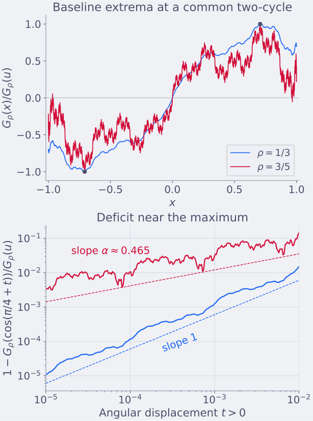
The two baseline series and their deficits near $u=1/\sqrt{2}$. The second panel uses the angular displacement $t$, with $x=\cos (\pi /4+t)$. The reference slopes illustrate the exit-scale estimates below; they are not fitted exponents. The plot is a finite-series illustration, not a certificate of a supremum or a minimax identity.

🏷️ The three counterexamples

The combined manuscript constructs three different functions. Its main assertions can be stated together. (Zhong, 2026)

Three continuous failures of symmetry inference

There exist functions $f_0,f_{\mathrm{o}},f_{\mathrm{e}}\in C(I)$ with these properties:

• $f_0(0)=0$ and $(P_n{f}_0)(0)=0$ for every $n\ge 0$, but $f_0$ is not odd.
• $f_{\mathrm{o}}(0)=0$ and $P_{2k+1}{f}_{\mathrm{o}}=P_{2k+2}{f}_{\mathrm{o}}$ for every $k\ge 0$, but $f_{\mathrm{o}}$ is not odd.
• $P_{2k}{f}_{\mathrm{e}}=P_{2k+1}{f}_{\mathrm{e}}$ for every $k\ge 0$, but $f_{\mathrm{e}}$ is not even.

In Saff and Varga’s numbering these refute Conjectures $1$, $3^{\prime }$, and $4$ for continuous functions. They do not assert that a single function satisfies all three sets of conditions.

All best approximants vanish at zero

The first construction is

$$\begin{array}{c}{h}_0=T_4-1-2T_5+{\beta }_0{T}_7,\\ f_0={\mathcal{S}}_{1/3}(T_3+\epsilon h_0).\end{array}$$

Here ${\beta }_0$ is a real algebraic number between $0.419$ and $0.420$.

Exact definition of the coefficient

Set $z=2\cos (\pi /36)$. The coefficient is defined by

$$\begin{array}{rl}107{\beta }_0=& -60+82z\\ & +1086z^2+1576z^3\\ & -2932z^4-3433z^5\\ & +2002z^6+2243z^7\\ & -510z^8-587z^9\\ & +44z^{10}+54z^{11}.\end{array}$$

The exact expression matters: the contact equations are equalities, and replacing ${\beta }_0$ by a rounded decimal does not preserve their proof.

The baseline is $F_0=G_{1/3}\circ T_3$. Oddness gives $P_0{G}_{1/3}=0$, while the approximation recurrence gives $P_1{G}_{1/3}=P_2{G}_{1/3}=T_1$. Composition then gives the seven initial approximants

$$P_n{F}_0=\{\begin{array}{ll}0,& 0\le n\le 2,\\ T_3,& 3\le n\le 6.\end{array}$$

Their residuals are $G_{1/3}\circ T_3$ and $-G_{1/3}\circ T_9/3$. Since the extrema of $G_{1/3}$ occur only at $\pm u$, the full contact sets are the zeros of $T_6$ and $T_{18}$, respectively.

Writing $H_0={\mathcal{S}}_{1/3}{h}_0$, the finite certificate supplies corrections $v_n\in {\mathcal{P}}_n$, all satisfying $v_n(0)=0$, and slopes ${\lambda }_n>0$. It proves that

$$\begin{array}{c}{P}_n{f}_0=P_n{F}_0+\epsilon v_n,\\ 0\le n\le 6.\end{array}$$

for the permitted perturbation sizes. The degree-seven functional equation then proves the origin condition for every $n$.

The asymmetry is visible at the two-cycle itself:

$$f_0(u)+f_0(-u)=-3\epsilon .$$

Indeed, the even part of $h_0$ is $T_4-1$, which equals $-2$ at both cycle points. The reflected sum of $H_0$ is therefore $-4{\sum }_{j\ge 0}(-1/3{)}^j=-3$. For every positive $\epsilon$ this rules out oddness. The manuscript proves the sufficient range

$$0<\epsilon \le \frac{1}{25000000}.$$

Equal approximants at odd/even degree pairs

For this construction use $\rho =3/5$ and

$$\begin{array}{c}{f}_{\mathrm{o}}={\mathcal{S}}_{\rho }(T_3+\epsilon h_{\mathrm{o}}),\\ \begin{array}{rl}{h}_{\mathrm{o}}=& (\eta -\sqrt{3}-1)T_0-\sqrt{3}{T}_2\\ & +T_4-3T_5+\eta T_6+{\beta }_{\mathrm{o}}{T}_7.\end{array}\end{array}$$

The exact algebraic coefficients are specified in the manuscript and odd certificate; their approximate values are $\eta =-1.5648142868\dots$ and ${\beta }_{\mathrm{o}}=-5.9148761843\dots$. The subscript distinguishes this coefficient from ${\beta }_0$ above. One of them has the relatively short formula

$$\begin{array}{rl}15\eta =& 16\cos (\pi /18)-26\cos (\pi /6)\\ & -26\cos (5\pi /18).\end{array}$$

The forcing satisfies $h_{\mathrm{o}}(0)=0$, so the functional equation gives $(1+\rho )f_{\mathrm{o}}(0)=0$. The finite certificates produce

$$\begin{array}{rl}{P}_1{f}_{\mathrm{o}}=P_2{f}_{\mathrm{o}}& =\epsilon v_1,\\ P_3{f}_{\mathrm{o}}=P_4{f}_{\mathrm{o}}& =T_3+\epsilon v_3,\\ P_5{f}_{\mathrm{o}}=P_6{f}_{\mathrm{o}}& =T_3+\epsilon v_5,\end{array}$$

where $\mathrm{deg}{v}_j\le j$. There are respectively four, six, and eight alternating contacts, sufficient for the higher degree in each pair. Cubic reduction supplies all subsequent pairs.

Since $T_3$ fixes both endpoints, the endpoint values of a series satisfy $({\mathcal{S}}_{\rho }h)(\pm 1)=h(\pm 1)/(1+\rho )$. Thus

$$f_{\mathrm{o}}(1)+f_{\mathrm{o}}(-1)=\frac{5}{2}\epsilon (\eta -\sqrt{3})\ne 0.$$

Normalization removes an additive constant as an explanation for this failure of oddness.

Equal approximants at even/odd degree pairs

The third construction starts from an even baseline:

$$f_{\mathrm{e}}={\mathcal{S}}_{3/5}(T_6+\epsilon h_{\mathrm{e}}).$$

The degree-eight forcing mixes parities. Write

$$h_{\mathrm{e}}=\sum _{k\in \{1,2,3,4,5,7,8\}}{c}_k{T}_k.$$

Its coefficients, four correction polynomials $w_0,w_2,w_4,w_6$, and four error corrections are the unique solution of an explicit $27\times 27$ algebraic linear system. The equations prescribe residual values at selected contacts, together with the normalizations $[T_2]w_2=1$ and $[T_4]w_4=-1$. Here $[T_j]w$ means the coefficient of $T_j$ in $w$. The manuscript specifies the system, and the even certificate stores its exact solution.

The four initial plateaus are

$$\begin{array}{rl}{P}_0{f}_{\mathrm{e}}=P_1{f}_{\mathrm{e}}& =\epsilon w_0,\\ P_2{f}_{\mathrm{e}}=P_3{f}_{\mathrm{e}}& =\epsilon w_2,\\ P_4{f}_{\mathrm{e}}=P_5{f}_{\mathrm{e}}& =\epsilon w_4,\\ P_6{f}_{\mathrm{e}}=P_7{f}_{\mathrm{e}}& =T_6+\epsilon w_6.\end{array}$$

The baseline contact sets are the zeros of $T_{12}$ for the first three pairs and of $T_{36}$ for the last pair. Exact bounds give $c_1+c_3+c_5+c_7>1/100$, so

$$\begin{array}{c}{f}_{\mathrm{e}}(1)-f_{\mathrm{e}}(-1)\\ =\frac{2\epsilon }{1+3/5}(c_1+c_3+c_5+c_7)\\ >\frac{\epsilon }{80}>0.\end{array}$$

This proves failure of evenness. For both plateau constructions the manuscript verifies the explicit choice $\epsilon =10^{-10}$.

🏷️ From finite contacts to a uniform certificate

The remaining issue is essential. Checking a residual at finitely many points does not by itself control its supremum between those points.

Let $p^0$ be a known baseline approximant, with residual $R=F-p^0$ and positive norm $E$. Its contact set is

$$S=\{\xi \in I:|R(\xi )|=E\}.$$

At a contact define $\sigma (\xi )=R(\xi )/E\in \{-1,1\}$. For a candidate correction $v$, put $D=H-v$. A finite certificate supplies a scalar $\lambda$ such that

$$\sigma (\xi )D(\xi )\le \lambda (\xi \in S).$$

The nonnegative difference $\lambda -\sigma (\xi )D(\xi )$ is the slack. A zero slack is an active contact, where the perturbed residual has the intended signed value $E+\epsilon \lambda$. Enough alternating active contacts prove bestness, provided one also proves

$$\Vert R+\epsilon D{\Vert }_{\infty }\le E+\epsilon \lambda .$$

The two parameter choices establish this uniform bound by related but distinct estimates.

Linear cusps for the origin construction

For a base degree $0\le n\le 6$, write $R_n=F_0-P_n{F}_0$, $E_n=\Vert R_n{\Vert }_{\infty }$, and $D_n=H_0-v_n$. Separate contacts by their sign:

$$\begin{array}{c}{S}_{n,s}=\{\xi :R_n(\xi )=s{E}_n\},\\ s\in \{-1,1\}.\end{array}$$

The manuscript proves two bounds, valid for every $x\in I$ and every contact $\xi \in S$:

$$\begin{array}{c}{E}_n-s{R}_n(x)\ge \mathrm{dist}(x,S_{n,s})/250,\\ |D_n(x)-D_n(\xi )|\le 10^5|x-\xi |.\end{array}$$

The second estimate is relative to each fixed contact. It does not assert that $H_0$ is globally Lipschitz between arbitrary pairs of points.

Choose a nearest contact $\xi \in S_{n,s}$ and put $d=|x-\xi |$. The finite inequality and the two analytic estimates combine into

$$\begin{array}{rl}& s(R_n(x)+\epsilon D_n(x))\\ & \le E_n-\frac{d}{250}\\ & +\epsilon ({\lambda }_n+10^{5}d)\\ & =E_n+\epsilon {\lambda }_n\\ & -\left(\frac{1}{250}-10^5\epsilon \right)d.\end{array}$$

For $\epsilon \le 1/25000000$, the final term is nonpositive. Applying both signs gives the required absolute bound. At active contacts equality remains exact, so alternation identifies the approximants.

Why does the perturbation admit a contact-relative linear bound? Pair its series as

$$\begin{array}{c}{H}_0=\sum _{j\ge 0}{9}^{-j}Q\circ T_{9^j},\\ Q=h_0-\frac{1}{3}{h}_0\circ T_3.\end{array}$$

The forcing was chosen so that $Q^{\prime }(u)=Q^{\prime }(-u)=0$. Near a cycle point, the terms before the exit scale are therefore bounded quadratically in the expanded displacement. The terms after that scale form a geometric tail. Both contributions are of order $|t|$. A finite number of applications of the functional equation transfers the estimate to the preimages that form the contact grids.

Thus self-similarity does two jobs in this example: it propagates the finite degree identities, and it provides a quantitative way to compare the baseline and perturbation at every scale.

Stronger cusps for the plateau constructions

For $\rho =3/5$, stationarity of the perturbation is unnecessary. Let $0<|t|\le \delta =1/16$, and choose $J$ to be the first nonnegative integer with $3^J|t|\ge \delta$. Then

$$\delta \le 3^J|t|\le 3\delta .$$

The positive-deficit resolvent formula gives

$$B-G_{3/5}(\cos (\pi /4+t))\ge \frac{{\rho }^J}{4608}.$$

The selected scale has moved the angle a definite distance away from the maximum. Its coefficient is comparable to ${\rho }^J$, and all the other deficits are nonnegative.

For an arbitrary polynomial forcing $h$, define

$$\begin{array}{c}M=\Vert h{\Vert }_{\infty },\\ L=\underset{\theta }{\sup }\left|\frac{d}{d\theta }h(\cos \theta )\right|.\end{array}$$

Splitting $H={\mathcal{S}}_{\rho }h$ at the same scale gives

$$\begin{array}{rl}& |H(\cos (\theta +t))-H(\cos \theta )|\\ & \le L|t|\sum _{j<J}(3\rho {)}^j\\ & +2M\sum _{j\ge J}{\rho }^j\\ & \le C{\rho }^J.\end{array}$$

The first sum is geometric because $3\rho =9/5>1$, and $|t|3^J$ is bounded. Subtracting a polynomial correction $v$ contributes at most a constant times $|t|$, which is also bounded by a constant times ${\rho }^J$.

Both the baseline deficit and perturbation oscillation are therefore measured on the same scale. In terms of distance, that scale is

$$\begin{array}{c}{\rho }^J\asymp |t{|}^{\alpha },\\ \alpha =\frac{\log (5/3)}{\log 3}\approx \mathrm{0.465.}\end{array}$$

This is the motivation for changing the contraction parameter. At $\rho =1/3$, the elementary bound for an arbitrary forcing gives $J|t|$, with a logarithmic loss. The origin construction removes that loss by stationarity of $Q$. At $\rho =3/5$, a geometric sum directly yields the required comparison for any polynomial forcing. The larger small-scale deficit permits more flexibility in solving the plateau contact equations.

For a baseline residual $R=sA{G}_{3/5}\circ T_d$, with $A>0$, the manuscript makes this comparison quantitative. If $\Vert v{\Vert }_{\infty }\le V$ and its angular derivative is bounded by $L_v$, set

$$\begin{array}{c}{C}_d=5M+\frac{15L}{64d}+\frac{3L_v}{16d},\\ K=\frac{5}{2}M+V,\gamma =\frac{1}{8\cdot 1296^2}.\end{array}$$

Sufficient smallness conditions are

$$\begin{array}{c}\epsilon C_d\le \frac{A}{4608},\\ \epsilon (K+|\lambda |)\le A\gamma .\end{array}$$

The first controls the matching signed residual near each contact. The second preserves its sign there and controls the error outside the contact neighborhoods, where the baseline has a fixed positive gap. This also allows negative $\lambda$: the total error $AB+\epsilon \lambda$ stays positive.

The certificate bounds give $C_d<178$, $K+|\lambda |<144$, and $A\ge 3/5$ in all seven plateau cases. They verify both inequalities for $\epsilon =10^{-10}$. Thus the finite table of slacks becomes an actual whole-interval minimax certificate.

🏷️ Exact algebra and finite orbits

The contact calculations do not approximate the infinite series by long truncations. On each contact grid, iteration by $T_3$ enters a short periodic orbit. The functional equation therefore determines the series values by a finite linear system.

For example, on the odd plateau grid, two iterates reach $\{u,-u\}$. At a grid point $x$, the exact value of ${\mathcal{S}}_{\rho }{T}_k$ is

$$\begin{array}{rl}({\mathcal{S}}_{\rho }{T}_k)(x)=& T_k(x)-\rho T_{3k}(x)\\ & +\frac{{\rho }^2}{1+(-1{)}^k\rho }{T}_{9k}(x).\end{array}$$

The denominator sums the alternating tail around the two-cycle, including the parity of $T_k$. In the even plateau construction the relevant orbits have eventual period dividing four, giving a denominator $1-{\rho }^4$ instead.

For the common-origin and odd plateau constructions, all grid and coefficient data lie in $\mathbb{Q}(z)$, with $z=2\cos (\pi /36)$ satisfying

$$\begin{array}{rl}m(z)=& z^{12}-12z^{10}\\ & +54z^8-112z^6\\ & +105z^4-36z^2+1=0.\end{array}$$

The even plateau construction uses $w=2\cos (\pi /72)$, satisfying $m(w^2-2)=0$. An algebraic number is represented by a rational coefficient list modulo its defining polynomial, together with a rational interval selecting the intended real root.

Polynomial reduction checks equalities exactly. Rational interval evaluation checks signs and positive margins. The data verify contact values, node order, the cubic node map, active equalities, inactive slacks, alternation, coefficient bounds, and explicit asymmetry witnesses. A tiny floating-point residual would establish none of the exact zero-slack identities required here.

There is still an analytic obligation after these finite checks: identify the stored values with the actual infinite series and prove persistence between the grid points. The preceding estimates provide that obligation, and the Lean development connects these parts explicitly.

flowchart TD
    A[Polynomial forcing<br/>and convergent series]
    B[Exact contact equations<br/>on finite orbits]
    C[Local gap estimates<br/>give uniform persistence]
    D[Alternation proves<br/>the initial minimizers]
    E[Cubic recurrence<br/>proves all degree conditions]
    F[An explicit witness<br/>rules out symmetry]
    A --> B --> C --> D --> E --> F

🏷️ Scope of the Lean proofs

The repository contains complete proofs of all three existence theorems. The final declarations construct the function, prove continuity on $I$, prove the required normalization where applicable, exhibit a failure of symmetry inside $I$, and establish the approximation conditions at every degree. The plateau conclusions include existence and uniqueness of the common best polynomial.

The definition of bestness is concrete. HasErrorBound f p E means $|f(x)-p(x)|\le E$ for every $x\in I$. Then IsBest f n p requires $\mathrm{deg}p\le n$ and says that every uniform error bound attained by any competitor of degree at most $n$ is also attained by $p$. On this compact interval, for continuous $f$, this is equivalent to minimizing the uniform norm. No best-approximation operator or analytic persistence hypothesis is assumed in the final results.

The endpoints are in Counterexample.lean, OddCounterexample.lean, and EvenCounterexample.lean. The checked finite identities use exact rational arithmetic; external Python calculations supply no mathematical assumptions.

Existence versus explicit perturbation sizes

The Lean endpoints choose a sufficiently small positive real $\epsilon$ from thresholds whose existence is proved in the development. They do not certify the manuscript’s particular numerical choices. The written proof establishes $0<\epsilon \le 4\times 10^{-8}$ for the common-origin construction and $\epsilon =10^{-10}$ for the two plateau constructions. These are distinct levels of quantitative specification of the same construction families.

The independent statement file imports only Mathlib and contains three intentional statement holes; Solution.lean proves the matching statements from the development. Those challenge holes are outside the proved dependency closure. The recorded axiom audit lists only propext, Classical.choice, and Quot.sound. The recorded definition comparison additionally checks the concrete approximation definitions, with no definition holes.

This post uses repository revision 2a1df364. Its Lean proof sources match the earlier successful verification run, which built the project, audited axioms, and ran the statement comparison with Lean, NanoDa, and con-ron on the pinned Lean/Mathlib v4.35.0-rc2 toolchain. For this post, the source hashes and three independent exact certificate checks were verified locally; the full Lean build and kernel replay are the linked repository verification, not a new local replay. At this revision the repository reports preparation for Palomar, with no registry submission or registration.

📊 Numerical illustration and exact checks

The figure script plots finite cosine series for the baselines and their deficits near a contact. It uses 60 terms. The omitted tail has the analytic bound

$${\Vert G_{\rho }-\sum _{j=0}^{N-1}(-\rho {)}^j{T}_{3^j}\Vert }_{\infty }\le \frac{{\rho }^N}{1-\rho }.$$

For $\rho =3/5$ and $N=60$, this is less than $1.3\times 10^{-13}$. That bound controls series truncation only, not floating-point phase evaluation. The illustration is separate from the exact certificate audits, which can be reproduced from the LorentzLean root with

python3 scripts/check_certificate.py
python3 certificates/plateau/audit_odd.py
python3 certificates/plateau/audit_even.py

The first reports 400 exact checks. The other two independently reconstruct and check the plateau certificates, including the explicit smallness inequalities. The degree reduction and persistence proofs explain why those finite calculations suffice for the infinite family of approximation conditions.

See Also

• on Lorentz Conjecture and best uniform approximation develops the earlier even-error and entire-function argument, including the necessity of retaining every odd-degree origin condition.
• on best uniform approximation from subspaces treats a different Lorentz question about choosing monomial approximation spaces; it provides further context for the role of alternation, but is not Conjecture 2 in Saff and Varga’s symmetry paper.

📚 References

🐻  Saff, E.B. & Varga, R.S. 1980. Remarks on some conjectures of G. G. Lorentz. Journal of Approximation Theory 30(1), 29–36.

🐻  Schoenberg, I.J. 1936. On the zeros of successive derivatives of integral functions. Transactions of the American Mathematical Society 40(1), 12–23.

🐻  Zhong, Y. 2026. Self-similar counterexamples to three conjectures of Lorentz.