Local smoothing in every dimension through an auxiliary determinant equation

Overview

A wave can concentrate sharply at one time. Local smoothing asks how much that concentration diminishes when measured over a time interval. OpenAI’s October 25, 2026 manuscript presents a proof of the Euclidean local smoothing conjecture in every spatial dimension, using a positive conserved wave current and an auxiliary nonlinear Dirichlet problem.

The mechanism for passing to higher dimensions is particularly striking: a determinant with one prescribed direction of curvature produces exactly the critical exponent $2n/(n-1)$, while the last propagation argument always takes place in one physical time variable and two auxiliary variables. The manuscript also extends the construction to a specified class of curved symmetric systems. This post develops those mechanisms and the resulting restriction and Kakeya estimates. (OpenAI, 2026)

🏷️ Half-waves and the local smoothing problem

Let $n\ge 2$ be the spatial dimension. For a Schwartz function $f:{\mathbb{R}}^n\to \mathbb{C}$, use the Fourier transform

$$\hat{f}(\xi )={\int }_{{\mathbb{R}}^n}{e}^{-iX\cdot \xi }f(X)dX.$$

The half-wave propagator is

$$\begin{array}{c}U(T)f=e^{-iT|D|}f,\\ U(T)f(X)\\ =\frac{1}{(2\pi {)}^n}{\int }_{{\mathbb{R}}^n}{e}^{i(X\cdot \xi -T|\xi |)}\hat{f}(\xi )d\xi ,\end{array}$$

where $|D|=\sqrt{-\Delta }$. It solves ${\partial }_T^{2}u-{\Delta }_{X}u=0$ with initial position $f$ and initial velocity $-i|D|f$. The other sign of the half-wave has the same estimates by complex conjugation.

Write $J=(1-\Delta {)}^{1/2}$ and define the Bessel-potential Sobolev norm by

$$\Vert f{\Vert }_{W^{s,p}}=\Vert J^{s}f{\Vert }_{L^p({\mathbb{R}}^n)}.$$

At frequency $|\xi |\asymp N$, this measures approximately $N^s\Vert f{\Vert }_p$. Here $A\asymp B$ means that their ratio is bounded above and below by positive constants independent of the frequency scale.

At a fixed nonzero time, wave propagation on $L^p$, $2\le p<\infty$, requires the derivative order

$$s_{\mathrm{fixed}}(p)=(n-1)\left(\frac{1}{2}-\frac{1}{p}\right).$$

Local smoothing replaces that single-time norm by

$$\begin{array}{c}\Vert U(T)f{\Vert }_{L_{X,T}^p}\\ ={\left({\int }_1^2\Vert U(T)f{\Vert }_p^{p}dT\right)}^{1/p}.\end{array}$$

Throughout this post, an unqualified spacetime norm uses $T\in [1,2]$; the data norm is spatial. Define

$$\begin{array}{rl}{p}_c& =\frac{2n}{n-1},\\ s_{+}(p)& =\max \left\{0,\frac{n-1}{2}-\frac{n}{p}\right\}.\end{array}$$

For $p\ge p_c$, the difference $s_{\mathrm{fixed}}(p)-s_{+}(p)$ is $1/p$. Below $p_c$, subtracting $1/p$ would give a negative order, so the conjectured threshold is instead zero.

Local smoothing stated in the manuscript

For every $n\ge 2$, $2\le p<\infty$, and $\epsilon >0$,

$$\begin{array}{c}\Vert U(T)f{\Vert }_{L_{X,T}^p}\\ \le C_{n,p,\epsilon }\Vert J^{s_{+}(p)+\epsilon }f{\Vert }_p.\end{array}$$

At $p=2$, one may take $\epsilon =0$. This is Theorem 1.1 of (OpenAI, 2026).

Thus the theorem gives every smoothing gain strictly less than $1/p$ above the critical exponent. The statement with an arbitrary positive $\epsilon$ must be kept distinct from an estimate at the exact Sobolev order $s_{+}(p)$.

The two-dimensional conjecture was proved by Guth, Wang, and Zhang through a sharp cone square-function estimate, first posted in 2019 and published in 2020. Their cone lies in ${\mathbb{R}}^3$ because it includes the time coordinate. (Guth, Wang & Zhang, 2020) In general spatial dimension $n$, Bourgain–Demeter cone decoupling supplies the full gain up to $\epsilon$ for $p\ge 2(n+1)/(n-1)$, leaving a gap to $p_c=2n/(n-1)$. (Bourgain & Demeter, 2015)

The earlier three-dimensional OpenAI note concerns a different manuscript and an argument through packet energies and entropy. The October 25 paper develops the auxiliary determinant method directly for general $n$.

🏷️ The critical estimate on a frequency annulus

Let $\phi$ be a smooth function with compact support away from the origin, and put $P_N=\phi (D/N)$. This is a smooth localization to frequencies comparable to $N$.

Critical annular estimate

Theorem 1.2 of the manuscript states that, for $N\ge 2$,

$$\begin{array}{rl}& \Vert U(T)P_{N}f{\Vert }_{L_{X,T}^{p_c}}\\ & \le C_{n,\phi }[\log (2+N){]}^{2/p_c}\Vert f{\Vert }_{p_c}.\end{array}$$

The constant is independent of $N$. It may depend on the spatial dimension. (OpenAI, 2026)

The logarithm is stronger information than an unspecified $N^{\epsilon }$ loss. It is also essential to the endpoint discussion: the paper gives a lower bound with logarithmic power $1/p_c$, leaving a gap between $1/p_c$ and $2/p_c$ for unrestricted data on a full annulus.

Spatial dimension $n$	Critical exponent $p_c$	Necessary log power	Proved log power in the manuscript
$2$	$4$	$1/4$	$1/2$
$3$	$3$	$1/3$	$2/3$
$4$	$8/3$	$3/8$	$3/4$
General $n$	$2n/(n-1)$	$(n-1)/(2n)$	$(n-1)/n$

Interpolation and frequency summation

Plancherel gives a uniform $L_X^2\to L_{X,T}^2$ estimate. At the other end, the annular wave kernel has $L^1$ norm $O(N^{(n-1)/2})$, giving an $L^{\infty }$ estimate with that cost.

For $p\ge p_c$, interpolation gives a frequency power

$$\frac{n-1}{2}\left(1-\frac{p_c}{p}\right)=\frac{n-1}{2}-\frac{n}{p}.$$

Interpolation between $2$ and $p_c$ introduces no positive power of $N$. Writing $L_N=\log (2+N)$, the annular bounds take the form

$$\begin{array}{c}\Vert U(T)P_{N}f{\Vert }_{L_{X,T}^p}\\ \lesssim N^{s_{+}(p)}{L}_N^{\beta (p)}\Vert f{\Vert }_p,\\ \beta (p)\\ =\min \left\{(n-1)\left(1-\frac{2}{p}\right),\frac{2}{p}\right\}.\end{array}$$

On dyadic frequencies $N=2^j$, inserting $\epsilon$ extra derivatives leaves the summable coefficients

$$2^{-j\epsilon }(1+j{)}^{\beta (p)}.$$

This proves the Sobolev theorem from the critical annular estimate. The new work lies in establishing that estimate at $p_c$.

🏷️ Gaussian localization from an imaginary translation

Set $d=n-1$ and $h=N^{-1}$. Initially work with a finite Fourier sum on a fixed spatial torus, and assume the frequencies lie in one small angular cap. The finite sum permits analytic continuation without convergence difficulties. The passage back to ${\mathbb{R}}^n$ comes later.

Translate a plane wave by an imaginary displacement along a light ray:

$$\begin{array}{c}(T,X)⟼(T-i\ell ,X-i\ell \omega ),\\ |\omega |=1,\ell >0.\end{array}$$

The multiplier introduced by this translation is exactly

$$\begin{array}{c}{e}^{\ell (\xi \cdot \omega -|\xi |)}\\ =\exp \left(-\frac{\ell |\xi |}{2}{\left|\omega -\frac{\xi }{|\xi |}\right|}^2\right).\end{array}$$

It is a Gaussian in the angular mismatch. When $N\ell \gg 1$, its angular width is approximately $(N\ell {)}^{-1/2}$. The important operation is to filter and sum the complex amplitudes before squaring. Squaring each mode separately would lose the interference responsible for focusing.

The symmetric system behind the Gaussian

Choose a spatial axis and write $X=(x,b)$ with $x\in {\mathbb{R}}^d$. Introduce null coordinates

$$t=\frac{T+b}{\sqrt{2}},s_0=\frac{b-T}{\sqrt{2}}.$$

The wave equation becomes

$$(2{\partial }_t{\partial }_{s_0}+{\Delta }_x)\psi =0.$$

A mode in the cap can be written as

$$\begin{array}{c}{u}_{\kappa ,v}=c_{\kappa ,v}{e}^{i\kappa (s_0+v\cdot x-|v{|}^{2}t/2)},\\ \kappa =\frac{{\xi }_b+|\xi |}{\sqrt{2}}>0,\\ v=\frac{{\xi }_x}{\kappa }\in {\mathbb{R}}^d.\end{array}$$

The first-order state $({\partial }_{s_0}\psi ,{\nabla }_x\psi )$ has $n$ components. Its symmetric system has characteristic polarization $E(v)=(1,v{)}^{\mathsf{T}}$. At the covector of this mode, its symbol $C(p)$ satisfies

$$\begin{array}{c}-w^{\mathsf{T}}C(p)w=\kappa |w^{\prime }-v{w}_0{|}^2,\\ w=(w_0,w^{\prime })\in \mathbb{R}\times {\mathbb{R}}^d.\end{array}$$

This is the algebraic origin of the positive angular Gaussian. Pairing two auxiliary real states into a complex state $(R,\zeta )$ gives the factor

$$\exp \left(-\frac{\kappa }{2}|\zeta -vR{|}^2\right).$$

The bilinear conservation law of the symmetric system then produces two auxiliary flows. Taking their real squares gives a positive semidefinite tensor with divergence-free columns. A holomorphic change of auxiliary coordinates puts that tensor into a form adapted to the physical time and spatial variables. These are the contents of Lemma 2.1 and Proposition 2.2 of the manuscript; positivity and conservation are both needed in the next stage.

🏷️ The conserved current and its spatial fibers

For each real spacetime coordinate, the construction introduces an auxiliary pair of real coordinates. Write the auxiliary time as $\tau \in \mathbb{C}$ and the auxiliary spatial coordinates as $(P,Z)\in {\mathbb{C}}^d\times \mathbb{C}$. The auxiliary complex structure is separate from the Fourier imaginary unit.

The useful coordinate functions are

$$\begin{array}{rlrl}Y& =\frac{\tau +Z}{\sqrt{2}},& S_1& =\frac{Z-\tau }{\sqrt{2}},\\ W& =\frac{P}{Y},& \Phi & =S_1+\frac{P\cdot P}{2Y}.\end{array}$$

The dot product in $P\cdot P$ is complex bilinear. The ratio $W$ records an auxiliary direction; $\Phi$ is a passive coordinate, constant along the current. On the domains used below, $Y\ne 0$.

After the coordinate change, the current is encoded by a quaternionic Hermitian matrix

$$A^0=\chi {\chi }^{\ast }.$$

Here $\ast$ denotes quaternionic conjugate transpose. Each mode contributes its polarization times a Gaussian weight to the column $\chi$; its scalar weight is

$$\begin{array}{c}{m}_{\kappa ,v}\\ ={\left(\frac{\kappa }{|Y|}\right)}^{d/2}{e}^{-\kappa |Y||W-v{|}^2/2}.\end{array}$$

The matrix $A^0$ is positive, its associated real tensor has zero column divergence, and $(\partial \Phi )A^0=0$. Its time entry $A_{TT}^0=|{\chi }_T{|}^2$ retains the interference of the original wave. Recovering the wave from this entry uses an invertible multiplier on the chosen cap; it is not a pointwise identification with $|U(T)f{|}^2$.

Before averaging, the lifted real tensor is a sum of only four rank-one squares, so its full determinant vanishes. The auxiliary equation will instead use its time density to construct a separate spatial Hessian with a nonzero determinant.

A definition of the quaternionic Hessian

The quaternion units satisfy ${\mathbf{i}}^2={\mathbf{j}}^2={\mathbf{k}}^2=-1$ and $\mathbf{ij}=\mathbf{k}$. Their role here is to organize three real coordinate slots per index. They impose no restriction that the spatial dimension be three or four.

For coordinates $q_a=x_{a0}+\mathbf{i}{x}_{a1}+\mathbf{j}{x}_{a2}$ and a real function $v$, define

$$\begin{array}{c}{H}_{ab}(v)\\ =\sum _{\alpha ,\beta =0}^2{e}_{\alpha }\overline{e_{\beta }}\frac{{\partial }^{2}v}{\partial x_{a\alpha }\partial x_{b\beta }},\\ (e_0,e_1,e_2)=(1,\mathbf{i},\mathbf{j}).\end{array}$$

This is a Hermitian matrix, and $\mathrm{tr}H(v)=\Delta v$. The Moore determinant of a quaternionic Hermitian matrix is the product of its real eigenvalues, counted with quaternionic multiplicity. In particular, it has degree $n$ on an $n\times n$ matrix, rather than degree $4n$ as in the full real representation.

Two properties drive the argument. For a holomorphic map $F$ of the auxiliary complex coordinates,

$$H(|F{|}^2)=4(DF{)}^{\ast }DF.$$

Thus a scalar holomorphic $\Phi$ gives a Hessian of rank at most one. Also, the cofactor $C(H(v))$, defined as the derivative of the determinant, has divergence-free real columns. This second conservation law permits integration by parts in the nonlinear equation.

The moving spatial domain

Choose $a=Kh$ for a sufficiently large fixed $K$, and take $h$ small enough that $4a\le 1$. Fix $z=(T,\tau )$ with $a<s=|\tau |<4$. The fiber ${\Omega }_z$ consists of all real spatial points on the torus and auxiliary spatial points satisfying

$$\begin{array}{c}r=\frac{|W{|}^2}{w_0^2}+100|Q{|}^2-1<0,\\ Q=\frac{\Phi }{a},w_0=\frac{1}{10}.\end{array}$$

In $(W,Q)$ this is a fixed ellipsoid. Its expression in the original auxiliary spatial coordinates changes with $\tau$. In this domain $|Y|\asymp s$, and its auxiliary volume element satisfies

$$dPdZ\asymp a^2{s}^{2d}dWdQ.$$

The current is smoothed in the real spatial variables, cut off in $Q$, and given a small positive regularization. The resulting matrix $A$ remains positive and conserved. Its time density $\mu =A_{TT}$ is strictly positive, and

$$\begin{array}{c}A:H(|\Phi {|}^2)=0,\\ A:B=\mathrm{Re}\mathrm{tr}(AB).\end{array}$$

This orthogonality allows the proof to add curvature in the $\Phi$ direction without creating an interior contribution when paired with the current.

🏷️ The determinant equation produces the critical exponent

Let $H_{\mathrm{fib}}$ denote the $n\times n$ spatial block of $H$ at fixed $(T,\tau )$. Set $B_0=\lambda |\Phi {|}^2$, with $\lambda$ a sufficiently large scale-dependent parameter. The paper chooses $\lambda =h^{-30n}$ after normalizing the torus data in $L^2$.

On each fiber it solves

$$\begin{array}{c}{D}_u=H_{\mathrm{fib}}(B_0+u)>0,\\ \det D_u=\lambda \mu ,u{|}_{\partial {\Omega }_z}=0.\end{array}$$

This is the auxiliary nonlinear Dirichlet problem. It constructs a potential from the wave’s positive density. The solution satisfies $u\le 0$. Appendix A supplies existence, uniqueness, comparison, and smooth dependence on the moving fiber parameters; these are required for differentiating the energy later.

The spatial background

$$B_{\mathrm{fib}}=H_{\mathrm{fib}}(B_0)$$

has one nonzero eigenvalue $\beta \asymp \lambda$. Consequently,

$$\det (B_{\mathrm{fib}}+\alpha I)=(\beta +\alpha ){\alpha }^{n-1}.$$

For $\alpha \lesssim \lambda$, matching this determinant to $\lambda \mu$ gives

$$\alpha \asymp {\mu }^{1/(n-1)}.$$

This is the precise point at which the critical dimension-dependent exponent appears.

A local comparison calculation

Suppose $\mu \ge m>0$ throughout a small ball of radius $h$ contained in a fiber. The construction ensures $m^{1/(n-1)}\le \lambda$. With $\ell$ denoting distance from its center, consider

$$v_b={ϵ}_0{m}^{1/(n-1)}({\ell }^2-h^2),$$

where ${ϵ}_0>0$ is a small fixed constant. Since there are three real slots per spatial index,

$$H_{\mathrm{fib}}(v_b)=6{ϵ}_0{m}^{1/(n-1)}I.$$

The determinant identity gives

$$\det H_{\mathrm{fib}}(B_0+v_b)\le \lambda m\le \det D_u$$

when ${ϵ}_0$ is small enough. On the boundary of the ball, $u\le 0=v_b$. The comparison principle therefore yields $u\le v_b$ inside. At the center,

$$\begin{array}{rl}-u& \gtrsim h^2{m}^{1/(n-1)},\\ (-u)\mu & \gtrsim h^2{m}^{n/(n-1)}.\end{array}$$

The cap multiplier estimate makes $m$ a controlled multiple of the squared wave amplitude, with explicit frequency and auxiliary-radius factors. Thus the power of the wave detected by the potential-density product is

$$2\cdot \frac{n}{n-1}=p_c.$$

This explains the reuse in higher dimensions. The same determinant construction acquires $n-1$ unconstrained eigenvalue directions as $n$ changes, and those directions generate exactly the exponent required by local smoothing. Uniformity is needed in $h$ for each fixed $n$; no estimate uniform as $n\to \infty$ is asserted.

🏷️ A corrected energy cancels the indefinite determinant

The potential suggests the nonnegative quantity

$$X_0(z)={\int }_{{\Omega }_z}(-u)\mu d\zeta ,$$

where $d\zeta$ is ordinary volume in all real and auxiliary spatial variables. But differentiating $X_0$ in $z=(T,\tau )$ introduces the full Hessian, including its time row. Only its spatial block $D_u$ is positive.

To expose the obstruction, write

$$\begin{array}{rl}H(B_0+u)& =\left(\begin{array}{cc}\ell & c^{\ast }\\ c& D_u\end{array}\right)\\ & =\sigma e_T{e}_T^{\ast }+\Sigma ,\end{array}$$

with

$$\begin{array}{c}\sigma =\ell -c^{\ast }{D}_u^{-1}c,\\ \Sigma =\left(\begin{array}{cc}{c}^{\ast }{D}_u^{-1}c& c^{\ast }\\ c& D_u\end{array}\right)\ge 0.\end{array}$$

The Schur-complement identity and the spatial equation give

$$\det H(B_0+u)=\lambda \mu \sigma .$$

Because $A:H(B_0)=0$ and $A_{TT}=\mu$,

$$\begin{array}{c}A:H(u)\\ =A:\Sigma +{\lambda }^{-1}\det H(B_0+u).\end{array}$$

The first term is nonnegative; the second can have either sign. Controlling only the spatial determinant would not resolve this problem.

The manuscript cancels the second term by adding a determinant energy. Put

$$\begin{array}{rl}{D}_{\theta u}& =H_{\mathrm{fib}}(B_0+\theta u),\\ {\mathcal{E}}_z(u)& =\frac{1}{\lambda }{\int }_{{\Omega }_z}u{\int }_0^1\det D_{\theta u}d\theta d\zeta ,\\ \mathcal{F}(z)& =X_0(z)+{\mathcal{E}}_z(u).\end{array}$$

This segment integral is an analogue of the Aubin–Mabuchi energy: differentiating it with respect to the potential recovers the determinant density. Conservation of its cofactor makes the differentiated correction cancel the full determinant in ${\Delta }_z{X}_0$.

Energy balance and comparison

Propositions and lemmas in Section 4 of the manuscript give

$${\Delta }_z\mathcal{F}+{\int }_{{\Omega }_z}A:\Sigma d\zeta =\mathcal{B}(z),$$

where $\mathcal{B}$ is the nonnegative wave flux through the side of the fiber. Moreover,

$$\frac{n-1}{n+1}{X}_0\le \mathcal{F}\le \frac{n}{n+1}{X}_0.$$

Thus the correction preserves the potential’s ability to measure the critical wave norm. (OpenAI, 2026)

The boundary cancellation is part of the mechanism. The full Hessian of the fiber’s defining function has a null direction tangent to the boundary and annihilated by $H(B_0)$. The normal-normal cofactor coefficient is a determinant on the orthogonal complement of the normal. That restricted form retains the null direction, so its determinant vanishes. Consequently, the determinant correction contributes no boundary flux; the remaining flux comes from the wave current.

Proof of the energy comparison

Write $R_0=C(D_u):B_{\mathrm{fib}}$. Since $B_{\mathrm{fib}}$ has rank one, the determinant along the segment has only two terms:

$$\begin{array}{rl}\det D_{\theta u}& ={\theta }^n\det D_u\\ & +(1-\theta ){\theta }^{n-1}{R}_0.\end{array}$$

Define

$$I_0={\int }_{{\Omega }_z}(-u)R_{0}d\zeta \ge 0.$$

Integrating the two powers of $\theta$ gives

$$\mathcal{F}=\frac{n}{n+1}{X}_0-\frac{I_0}{\lambda n(n+1)}.$$

Let $q=G_{\mathrm{fib}}(u)$ be the spatial gradient written as a quaternionic column. The cofactor identity $C(D_u):D_u=n\det D_u$ and integration by parts give a nonnegative quantity

$$\begin{array}{c}{Q}_0=n\lambda X_0-I_0\\ ={\int }_{{\Omega }_z}{q}^{\ast }C(D_u)qd\zeta \ge 0.\end{array}$$

Substitution yields the exact identity

$$\begin{array}{rl}\mathcal{F}& =\frac{n-1}{n+1}{X}_0\\ & +\frac{Q_0}{\lambda n(n+1)}.\end{array}$$

Positivity proves the lower bound, while $I_0\ge 0$ proves the upper bound.

🏷️ Gaussian separation controls the boundary flux

Two estimates are needed: an upper bound on the flux at the fiber wall and a lower bound recovering the wave inside the fiber. Their exponential factors must be compared quantitatively.

The data lie in $|v|\le \gamma$ for a small fixed cap aperture $\gamma$. On the portion of the wall carrying wave flux, the cutoff in $Q$ forces $|W|$ to be bounded below by a fixed multiple of $w_0$. The angular mismatch is therefore bounded away from zero, and the Gaussian contributes

$$e^{-c_{0}s/h}.$$

Near the center, $|W|\le \gamma$, the Gaussian multiplier can be inverted to recover the wave. This costs an exponential of the form $e^{C{\gamma }^{2}s/h}$. The lower density estimate on wavelength-sized balls and the determinant comparison above yield

$$\begin{array}{c}\mathcal{F}(T,\tau )\\ {\gtrsim }_{\gamma }{a}^2(s/h{)}^{-M}{e}^{-C{\gamma }^{2}s/h}\Vert U(T)f{\Vert }_{p_c}^{p_c}\end{array}$$

for a fixed exponent $M$. A spatially averaged comparison potential also bounds the normal derivative of $u$ at the wall. Combining it with the Gaussian wall decay bounds the flux by the same wave norm, with exponential $e^{-c_{0}s/h}$ and polynomial scale factors.

Choose $\gamma$ so that $C{\gamma }^2<c_0/2$. Dividing the flux upper bound by the energy lower bound leaves a decaying exponential; it absorbs the polynomial factors. This produces the scalar differential inequality

$$\begin{array}{c}{\Delta }_{T,\tau }\mathcal{F}\le V(s)\mathcal{F},\\ V(s)=C{s}^{-2}{e}^{-cs/h},\\ 2a\le s\le 3.\end{array}$$

On the input circle $|\tau |=4a$ and the output circle $|\tau |=2a$, respectively, Section 5 obtains the matching estimates

$$\begin{array}{rl}\mathcal{F}(0,\tau )& \lesssim a^2\Vert f{\Vert }_{p_c}^{p_c},\\ \mathcal{F}(T,\tau )& \gtrsim a^2\Vert U(T)f{\Vert }_{p_c}^{p_c}.\end{array}$$

This comparison resolves a significant issue: localization suppresses the boundary current, but recovering the unfiltered wave also has a cost. The proof succeeds because the former exponential dominates the latter after the cap is chosen sufficiently small.

🏷️ Two annulus comparisons and the logarithmic loss

The remaining propagation takes place in

$$(T,\tau )\in \mathbb{R}\times {\mathbb{R}}^2,$$

regardless of the original dimension $n$. Let

$$M(T,s)=\frac{1}{2\pi }{\int }_0^{2\pi }\mathcal{F}(T,s{e}^{i\theta })d\theta$$

be the circular mean, and set $b=2a$, taking $h$ small enough that $b<1/4$.

The observation is on the thin cylinder $s=b$, $1\le T\le 2$, while the input controls $T=0$, $s=2b$. Section 6 compares them by moving outward to radius one, moving in physical time through a region of fixed size, and then moving inward again.

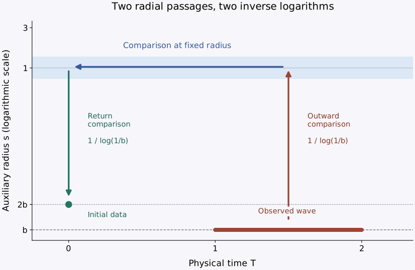
The arrows represent comparisons of a nonnegative scalar energy. They are not trajectories of the physical wave. The radial axis is logarithmic; $b$ is a small multiple of the wavelength.

The elementary source of a logarithm is the planar radial harmonic equation

$$v^{\prime \prime }(s)+\frac{1}{s}{v}^{\prime }(s)=0.$$

Its solution with $v(b)=0$, $v(1)=1$ is

$$v(s)=\frac{\log (s/b)}{\log (1/b)}.$$

At $s=2b$, its size is $\log 2/\log (1/b)$. Equivalently, this is the probability that planar Brownian motion started at radius $2b$ exits the annulus through its outer circle. Each passage between the small radius and a fixed radius costs one inverse logarithm.

The exponentially decaying potential preserves this comparison. The relevant uniform bound is

$${\int }_b^{3}s\log (s/b)V(s)ds\lesssim 1.$$

Indeed, substituting $s=bt$ and using $b=2Kh$ bounds it by a constant times

$${\int }_1^{\infty }\frac{\log t}{t}{e}^{-2cKt}dt.$$

Together with a mean-value comparison on the fixed outer region, the scalar cylinder lemma gives

$$\begin{array}{c}M(0,2b)\\ \gtrsim [\log (3/b){]}^{-2}{\int }_1^{2}M(T,b)dT.\end{array}$$

Insert the input and output energy bounds, cancel $a^2$, and take the $p_c$th root. The result is

$$\Vert U(T)f{\Vert }_{L_{X,T}^{p_c}}\lesssim [\log (2/h){]}^{2/p_c}\Vert f{\Vert }_{p_c}$$

on the torus for cap-localized data. Homogeneity removes the initial $L^2$ normalization. A finite covering by caps handles the full annulus. The remaining bounded frequency range is absorbed into the constant.

To return to ${\mathbb{R}}^n$, the proof localizes in physical space and periodizes the nearby data. Away from the wave cone, the frequency-localized kernel has rapidly decaying tails, obtained by integration by parts in frequency. Those tails control the difference between the periodic and Euclidean outputs. This completes the critical annular estimate, after which interpolation and dyadic summation give the Sobolev theorem.

The two logarithms are intrinsic to the scalar comparison used here: the manuscript constructs scalar supersolutions for which both losses occur. Improving the wave estimate to the lower logarithmic power would require exploiting further structure of the wave energy.

🏷️ Reuse for curved symmetric systems

The higher-dimensional theorem already concerns every Euclidean spatial dimension. Appendix E addresses a separate form of reuse: replacing the Euclidean phase $|\xi |$ by a curved characteristic sheet of a symmetric system.

A real symmetric matrix pencil is a linear matrix-valued function

$$\begin{array}{c}C(\xi )=\sum _{j=1}^n{\xi }_j{C}_j,\\ C_j\in {\mathbb{R}}^{n\times n},C_j^{\mathsf{T}}=C_j.\end{array}$$

Let $\varphi (\xi )$ be its largest eigenvalue. Assume on an open cone that this eigenvalue is simple and that $D^2\varphi (\xi )$ is positive definite on ${\xi }^{\perp }$. The radial direction is excluded because $\varphi$ is homogeneous of degree one.

Extension stated in Appendix E

For a smooth compactly supported multiplier $b_0$ inside that cone,

$$\begin{array}{rl}& \Vert e^{-iT\varphi (D)}{b}_0(hD)f{\Vert }_{L_{X,T}^{p_c}}\\ & \le C_{b_0}[\log (2/h){]}^{2/p_c}\Vert f{\Vert }_{p_c},\\ & 0<h\le 1.\end{array}$$

The constant may depend on the pencil. There is an analogous statement for a simple smallest eigenvalue with negative definite transverse Hessian. (OpenAI, 2026)

The assumptions provide concrete replacements for the wave geometry. With

$$S(\xi )=\varphi (\xi )I-C(\xi ),$$

the extremal eigenvalue ensures $S\ge 0$. Its null eigenvector provides the polarization, and its positive block on the complementary states provides the angular Gaussian. Transverse curvature makes the polarization a local coordinate on the angular patch. The construction then supplies a passive $\Phi$, the same rank-one background, and the same determinant energy.

More explicitly, fix a unit direction $\omega$ and let $e_0$ be its unit top eigenvector. Let $S_{\perp }$ be the restriction of $S(\omega )$ to $e_0^{\perp }$, and define $Lw$ as the projection of $C(w)e_0$ onto $e_0^{\perp }$. Differentiating the eigenvector equation gives, for $w\in {\omega }^{\perp }$,

$$\begin{array}{c}{D}^2\varphi (\omega )[w,w]\\ =2(Lw{)}^{\mathsf{T}}{S}_{\perp }^{-1}Lw,\\ Dv(\omega )w=S_{\perp }^{-1}Lw,\end{array}$$

where $(1,v(\xi ){)}^{\mathsf{T}}$ is the local eigenvector normalized in the $e_0$ direction. Positive transverse curvature makes $L$ injective. The equality between the number of state components and spatial variables now matters: both transverse spaces have dimension $n-1$, so $L$ and $Dv(\omega )$ are isomorphisms. This supplies the angular chart needed by the Gaussian and fiber construction. Curvature alone does not automatically supply all of these ingredients for an arbitrary phase or a variable-coefficient equation.

A characteristic sheet that is not quadratic

In three spatial dimensions, the paper considers

$$C(x,y,z)=\left(\begin{array}{ccc}z& x& y\\ x& -z& 0\\ y& 0& -2z\end{array}\right).$$

At $(0,0,1)$ the largest eigenvalue is $1$, is simple, and has transverse Hessian $\mathrm{diag}(1,2/3)$. The characteristic polynomial is

$$\begin{array}{rl}& (t-z)(t+z)(t+2z)\\ & -x^2(t+2z)-y^2(t+z).\end{array}$$

The paper shows it is irreducible. Its theorem therefore applies near this ray to a cubic characteristic sheet, beyond a linear change of coordinates in the ordinary wave cone.

🏷️ Sharpness and the remaining endpoint gap

The focusing example makes the threshold visible. Fix $T_0=3/2$ and choose a nonnegative smooth radial cutoff $\psi$ supported in $(5/4,7/4)$. Set

$${\hat{f}}_N(\xi )=e^{i{T}_0|\xi |}\psi (|\xi |/N).$$

At time $T_0$, the radial oscillation in the initial data is cancelled by propagation. At time $T_0+u$, stationary phase gives a large wave on a shell of radius approximately $u$ and thickness $N^{-1}$. Its volume is approximately $N^{-1}{u}^{n-1}$.

Combining the shell amplitude and volume with the initial-data norm yields the lower bound

$$\begin{array}{c}\frac{\Vert U(T)f_N{\Vert }_{L_{X,T}^p}^p}{\Vert f_N{\Vert }_p^p}\\ \gtrsim {\int }_{A/N}^{1/4}{u}^{(n-1)(1-p/2)}du\end{array}$$

for a fixed large $A$. At $p=p_c$, the exponent of $u$ is $-1$. Each dyadic distance from the focus contributes comparable mass, giving

$$\frac{\Vert U(T)f_N{\Vert }_{L_{X,T}^{p_c}}}{\Vert f_N{\Vert }_{p_c}}\gtrsim (\log N{)}^{1/p_c}.$$

For $p>p_c$, the same integral gives the necessary power $N^{(n-1)/2-n/p}$. Section 8 also gives a different packet construction showing that order-zero smoothing fails throughout $2<p\le p_c$, even with a weak spacetime norm.

Thus the strict Sobolev conjecture and the optimal logarithmic estimate are different questions. The manuscript resolves the former and leaves the unrestricted critical logarithmic exponent between $1/p_c$ and $2/p_c$. With any fixed positive angular regularity on the input, Appendix B obtains the lower power $1/p_c$; that additional hypothesis cannot simply be dropped.

🏷️ Restriction and Kakeya consequences

For a function $g$ on the unit sphere, its Fourier extension is

$$Eg(X)={\int }_{S^{n-1}}{e}^{iX\cdot \omega }g(\omega )d\sigma (\omega ).$$

To extract extension from smoothing, the paper modulates and averages the wave in time to isolate a thin frequency shell. Incoming spherical data of the form $e^{-iNr}\psi (r)g(\omega )$ cancel that shell’s radial phase near the focus. Rescaling space then recovers $Eg$. At $p_c$, the scaling factor is exactly balanced because $n/p_c=(n-1)/2$.

Section 9 obtains the local estimate

$$\begin{array}{rl}& \Vert Eg{\Vert }_{L^{p_c}(B(X_0,R))}\\ & \lesssim [\log (2+R){]}^{2/p_c}\Vert g{\Vert }_{L^{p_c}(S^{n-1})}.\end{array}$$

An epsilon-removal argument converts its subpolynomial growth into global estimates at strictly larger exponents. In the notation $1/a+1/a^{\prime }=1$, the resulting spherical extension range is

$$\begin{array}{c}\Vert Eg{\Vert }_{L^b({\mathbb{R}}^n)}\lesssim \Vert g{\Vert }_{L^a(S^{n-1})},\\ 1<a\le \infty ,b<\infty ,\\ b>\frac{2n}{n-1},b>\frac{n+1}{n-1}{a}^{\prime }.\end{array}$$

These are the interior inequalities; no boundary case follows merely by replacing the strict signs with non-strict ones.

For geometry, let $T_{\delta }(x,\omega )$ be a unit-length tube of radius $\delta$ centered at $x$ and parallel to $\omega$. Define the Kakeya maximal operator by

$$\begin{array}{c}{K}_{\delta }F(\omega )\\ =\underset{x}{\sup }\frac{1}{|T_{\delta }(x,\omega )|}{\int }_{T_{\delta }(x,\omega )}|F(y)|dy.\end{array}$$

A small frequency cap produces an extended wave concentrated on a long thin tube. Assigning random signs to disjoint caps turns estimates for their oscillatory sum into estimates for the sum of their squared amplitudes, hence for tube overlap. The paper tracks the logarithm through this argument and obtains

$$\begin{array}{rl}& \Vert K_{\delta }F{\Vert }_{L^n(S^{n-1})}\\ & \lesssim [\log (2/\delta ){]}^{4/p_c}\Vert F{\Vert }_{L^n({\mathbb{R}}^n)}.\end{array}$$

Since $4/p_c=2(n-1)/n$, this implies the conjectured ${\delta }^{-\epsilon }$ bound for every $\epsilon >0$. Applying the maximal estimate across the scales of a covering yields full Hausdorff dimension $n$ for every set containing a unit segment in each direction. A lower bound only on the volume of a fixed-radius neighborhood would not by itself establish this Hausdorff conclusion.

The remaining applications include the strict Bochner–Riesz multiplier range, maximal Bochner–Riesz estimates for $p\ge 2$, Stein’s square function, restriction for the truncated cone and compact paraboloid, and Schrödinger local smoothing. The two reusable inputs in these consequences are the critical annular estimate and the quantitative control of its logarithmic loss. (OpenAI, 2026)

🏷️ Release and verification scope

The October 26 announcement identifies the October 25 manuscript as the new release and reports a Lean formalization. The theorem statements and proof architecture above refer to that manuscript at repository snapshot 7ef5c0c.

The accompanying formalization scope page lists all-dimensional local smoothing, strict multiplier and extension estimates, Kakeya maximal estimates with ${\delta }^{-\epsilon }$ loss, and the Hausdorff-dimension conclusion. That scope statement is distinct from a claim that every quantitative refinement in the paper has been formalized. This exposition is based on the mathematical source; it does not constitute an independent complete proof audit or a Lean build and axiom audit.

See Also

• Critical local smoothing in three dimensions develops the earlier packet-energy approach and provides a comparison with the determinant method.
• on l2 decoupling theorem introduces the frequency decompositions behind the previous general-dimensional range.
• on boundary integral with stationary phase develops the oscillatory asymptotics used in the focusing example and the passage from spherical waves to extension.
• Kakeya tubes and dimension distinguishes maximal estimates, tube-volume bounds, and Hausdorff-dimension statements.
• Bochner–Riesz multipliers explains the difference between fixed-radius and maximal summation estimates.

🐻  Bourgain, J. & Demeter, C. 2015. The proof of the l² decoupling conjecture. Annals of Mathematics 182(1), 351–389.

🐻  Guth, L., Wang, H. & Zhang, R. 2020. A sharp square function estimate for the cone in ℝ³. Annals of Mathematics 192(2), 551–581.

🐻  OpenAI 2026. Local smoothing for the Euclidean wave equation.