on entry growth in Gaussian elimination

Overview

The growth factor of Gaussian elimination measures how much the elimination process can amplify matrix entries, and it controls the number of bits of precision a stable solve requires. Shah and Urschel (Shah & Urschel, 2026) resolve the asymptotic worst-case behavior of this quantity under the principal pivoting strategies, answering a question that has been open since Goldstine and von Neumann’s 1947 analysis of complete pivoting (von Neumann & Goldstine, 1947).

For row-only strategies the news is negative. Partial pivoting retains its exponential worst case $2^{n-1}$ even for sparse matrices: growth $2^{n-1}$ forces at least $4n-4$ nonzeros, and this is tight; with at most $k+1$ nonzeros per row and column, growth at least $r_k^{n-1}\ge (2-2^{1-k}{)}^{n-1}$ is still possible, where $r_k$ solves $x^k=x^{k-1}+\cdots +x+1$. Randomized partial pivoting fails as well: for every exponent $p\in (0,\infty )$ there are matrices on which it produces growth $e^{{\Omega }_p(n/\ln n)}$ with high probability. The positive counterpart is a randomized row-pivoting strategy based on volume sampling — a nested chain of projection determinantal point processes — which achieves $\mathbb{E}\mathrm{growth}(PA)\le (\frac{1}{\sqrt{6}}+o(1))n^2$ for every matrix. The catch is computational: deciding whether some row permutation keeps growth bounded is NP-hard, already at threshold $1$ with a constant gap of $\frac{3}{2}$.

The central results concern strategies that may permute rows and columns. Rook pivoting admits matrices with growth $n^{(\frac{1}{4}-o(1)){\log }_{2}n}$, within a factor of two in the exponent of Foster’s upper bound $\frac{3}{2}{n}^{\frac{3}{4}\ln n}$ (Foster, 1997). Complete pivoting admits matrices with growth $e^{\Omega ({\ln }^{2}n)}$, matching the quasi-polynomial form of Wilkinson’s 1961 upper bound $2\sqrt{n}{n}^{\frac{1}{4}\ln n}$ (Wilkinson, 1961) and its 2025 improvement $n^{0.2079\ln n+O(1)}$ (Bisain, Edelman & Urschel, 2025). The worst-case growth factor under complete pivoting is therefore $n^{\Theta (\ln n)}$: its order is now determined, closing the oldest open problem in numerical linear algebra.

Preprint status and provenance

The paper is arXiv v1 from August 20, 2026. The authors state that the mathematics has been checked for overall correctness, while noting that presentation will be improved before submission for publication.

The manuscript carries a section-by-section AI usage statement, disclosing that parts were developed in human—AI interaction with ChatGPT Sol 5.6 and Claude Fable 5. The sparse partial-pivoting results began as human work predating these systems and were sharpened through interaction. The volume-sampling section was proven with AI assistance around a human-generated determinantal point process idea. The NP-hardness proof grew out of a human proof of a related statement. The randomized-partial-pivoting analysis emerged from human—AI collaboration around a Jordan-block construction suggested through prompting. The rook-pivoting results were proven without AI, beginning in 2022. The complete-pivoting lower bound followed a research roadmap developed by the authors since 2022, whose execution the authors state AI accelerated considerably — by their estimate, possibly saving a year of human-only work — while noting that the systems could not have produced the result without that roadmap. The authors invite questions about disclosure methodology, observing that no standard norms exist.

🏷️ Preliminaries: Elimination, Norms, and Strategies

The elimination process and the growth factor

Gaussian elimination factors $A$ into a product $LU$ by a sequence of rank-one updates. Partition

$$A=\left(\begin{array}{cc}{M}^{(1,1)}& M^{(1,2)}\\ M^{(2,1)}& M^{(2,2)}\end{array}\right)$$

with $M^{(1,1)}$ the leading $k\times k$ block. Eliminating the first $k$ pivots leaves the Schur complement

$$A^{(k)}=M^{(2,2)}-M^{(2,1)}{\left[M^{(1,1)}\right]}^{-1}{M}^{(1,2)}.$$

The factorization is read off the first row and column of each iterate: $L_{ij}=A_{i-j+1,1}^{(j-1)}/A_{11}^{(j-1)}$ and $U_{ij}=A_{1,j-i+1}^{(i-1)}$. Throughout, $A[R,C]$ denotes the submatrix on row set $R$ and column set $C$, and $[k]=\{1,\dots ,k\}$. Two facts about this setup are used repeatedly below. First, every iterate is itself a Schur complement, so the recursive constructions of the rook and complete-pivoting lower bounds are designed around Schur complement identities; this is the algebraic content of Sylvester’s determinantal identity. Second, Cramer’s rule expresses the elimination coefficients as ratios of determinants of bordered submatrices, which is what makes determinantal distributions (volume sampling, determinantal point processes) the right probabilistic tool for analyzing pivoting.

The growth factor is

$$\mathrm{growth}(A)=\max \left(\Vert L{\Vert }_{\max },\frac{\Vert U{\Vert }_{\max }}{\Vert A{\Vert }_{\max }}\right),$$

where $\Vert \cdot {\Vert }_{\max }$ is the entrywise maximum absolute value. It measures the worst relative amplification of any entry during the factorization.

Norms and the cost of instability

Besides $\Vert \cdot {\Vert }_{\max }$, the analysis uses the Frobenius norm $\Vert \cdot {\Vert }_F$ and two operator norms: $\Vert A{\Vert }_{1\to 2}={\max }_{\Vert x{\Vert }_1\le 1}\Vert Ax{\Vert }_2$, the largest column ${\ell }^2$ norm, and $\Vert A{\Vert }_{2\to \infty }=\Vert A^{\top }{\Vert }_{1\to 2}$, the largest row ${\ell }^2$ norm. The elementary relations

$$\Vert \cdot {\Vert }_{\max }\le \Vert \cdot {\Vert }_F,\Vert A{\Vert }_{1\to 2}\le \sqrt{n}\Vert A{\Vert }_{\max }$$

bridge entrywise and averaged control throughout the paper.

Why the growth factor matters: backward error analysis shows that a computed LU factorization solves a nearby system, and the number of bits of precision a stable computation requires scales as $\log \mathrm{growth}(A)$ (Urschel, 2025). A growth factor of $2^{n-1}$ therefore destroys nearly all bits of double precision already for a $100\times 100$ Wilkinson matrix, and yet partial pivoting — which only exchanges rows — remains the default dense solver in essentially every programming language because it is cheap and rarely behaves badly in practice. This tension between provable worst cases and observed behavior is the motivating problem of the entire subject.

Pivoting strategies and two randomized rules

To control growth one replaces $A$ by $PAQ$ for permutation matrices $P,Q$ chosen by a pivoting strategy. For worst-case analysis it suffices to study matrices that require no pivoting under the strategy: if the rule always selects the $(1,1)$ entry of the current iterate, the strategy never permutes. This yields three classes of $n\times n$ real matrices, defined by the requirement on every iterate $A^{(k)}$:

$$\begin{array}{rlrl}{\mathrm{PP}}_n(\mathbb{R}):& \left|a_{11}^{(k)}\right|\ge \underset{j}{\max }\left|a_{j1}^{(k)}\right|& & \text{(partial)},\\ {\mathrm{RP}}_n(\mathbb{R}):& \left|a_{11}^{(k)}\right|\ge \underset{j}{\max }\max \left(\left|a_{1j}^{(k)}\right|,\left|a_{j1}^{(k)}\right|\right)& & \text{(rook)},\\ {\mathrm{CP}}_n(\mathbb{R}):& \left|a_{11}^{(k)}\right|\ge \underset{i,j}{\max }\left|a_{ij}^{(k)}\right|& & \text{(complete)}.\end{array}$$

The paper also analyzes two randomized strategies, viewed as distributions over permutation sequences $(r_1,\dots ,r_n)$. Volume pivoting has marginals

$$\mathrm{Pr}\left(\{r_1,\dots ,r_k\}=R\right)\propto \stackrel{2}{\det }A[R,[k]],$$

and randomized partial pivoting ${\mathrm{RPP}}_p$ has transition probabilities

$$\mathrm{Pr}\left(r_k=r|\{r_1,\dots ,r_{k-1}\}=R\right)\propto {\left|\frac{\det A[R+r,[k]]}{\det A[R,[k-1]]}\right|}^p,$$

which by Cramer’s rule reduce to ${\left|a_{r1}^{(k)}\right|}^p$, the $p$-th power of the leading entry of row $r$ in the current iterate. As $p\to \infty$ one recovers partial pivoting; as $p\to 0$, uniform random pivoting.

The historical baseline

The following table collects the landmarks preceding this paper; all bounds are worst-case over $n\times n$ matrices with $\Vert A{\Vert }_{\max }=1$.

Year	Authors	Result	Growth bound
1947	Goldstine—von Neumann	First stability analysis; complete pivoting introduced (von Neumann & Goldstine, 1947)	—
1961	Wilkinson	Upper bound for complete pivoting (Wilkinson, 1961)	$2\sqrt{n}{n}^{\frac{1}{4}\ln n}$
1965	Wilkinson	Worst case for partial pivoting (the Wilkinson matrix) (Wilkinson, 1965)	$2^{n-1}$ (sharp)
1989	Higham—Higham	Classification of all partial-pivoting extremals (Higham & Higham, 1989)	equality class
1991	Gould	Folklore conjecture $\mathrm{growth}\le n$ fails in dimension 13 (Gould, 1991)	$>n$ (floating point)
1992	Edelman	Same failure in exact arithmetic (Edelman, 1992)	$>n$ (exact)
1997	Foster	Upper bound for rook pivoting (Foster, 1997)	$\frac{3}{2}{n}^{\frac{3}{4}\ln n}$
2024	Edelman—Urschel	Conjecture fails for all $n\ge 11$; rook lower bound (Edelman & Urschel, 2024)	$n^{1.669}$
2025	Fedorovskii	Lower bound for complete pivoting (Fedorovskii, 2025)	$n^{{\log }_{7/2}4}\approx n^{1.107}$
2025	Bisain—Edelman—Urschel	First improvement of Wilkinson’s upper bound in six decades (Bisain, Edelman & Urschel, 2025)	$n^{0.2079\ln n+0.91}$
2026	Shah—Urschel	Lower bounds settling the order for rook and complete pivoting (Shah & Urschel, 2026)	$n^{(\frac{1}{4}-o(1)){\log }_{2}n}$, $e^{\Omega ({\ln }^{2}n)}$

Until this paper, the gap between lower and upper bounds was enormous for both column-permuting strategies: polynomial lower bounds against quasi-polynomial upper bounds. The new lower bounds close that gap.

🌵 Sparse Matrices Under Partial Pivoting

The Wilkinson matrix is only mildly sparse, with $3n-1$ nonzeros. Exponential growth nevertheless occurs in applications: Wright found sparse examples from two-point boundary value problems with at most three nonzeros per row and growth approaching $2^{n/2}$ (Wright, 1993), and Foster found examples from Volterra quadrature (Foster, 1994). Shah and Urschel determine exactly how sparse a matrix attaining the extremal growth can be.

Sparse exponential growth

For every $n>2$ there is $A\in {\mathrm{PP}}_n(\mathbb{R})$ with $\mathrm{nnz}(A)=4n-4$ and $\mathrm{growth}(A)=2^{n-1}$, and no matrix in ${\mathrm{PP}}_n(\mathbb{R})$ with growth $2^{n-1}$ can have fewer nonzeros. For every $k>1$ and $n\ge k+1$ there is $A\in {\mathrm{PP}}_n(\mathbb{R})$ with at most $k+1$ nonzeros per row and column and $\mathrm{growth}(A)=r_k^{n-1}\ge (2-2^{1-k}{)}^{n-1}$, where $r_k$ is the unique root of $x^k=x^{k-1}+\cdots +x+1$ in $(2-2^{1-k},2)$. Every matrix with at most two nonzeros per row and column has growth at most $2$.

The sharpness statement rests on the Higham—Higham characterization: every $A\in {\mathrm{PP}}_n(\mathbb{R})$ with growth $2^{n-1}$ has the form

$$A=DM\left[\begin{array}{cc}\left(\begin{array}{c}T\\ 0\end{array}\right)& \theta d\end{array}\right],d=(1,2,4,\dots ,2^{n-1}{)}^{\top },$$

where $D$ is a $\pm 1$ diagonal matrix, $M$ is unit lower triangular with $M_{ij}=-1$ for $i>j$, $T\in {\mathbb{R}}^{(n-1)\times (n-1)}$ is nonsingular upper triangular, and $\theta =|A_{1n}|=\Vert A{\Vert }_{\max }$. Setting $B:=D^{-1}A$, the first column of $B$ is a scalar multiple of the first column of $M$ (hence fully nonzero) and the last column is $\theta \cdot Md=\theta \cdot 1$ (since $Md=1$), contributing $2n$ nonzeros. Each interior column $j$ must carry at least two more: because $T$ is upper triangular,

$$T_{j+1,j}=e_{j+1}^{\top }{M}^{-1}B{e}_j=(2^{j-1},2^{j-2},\dots ,2,1,1,0,\dots ,0)B{e}_j=0.$$

All coefficients of this linear form are positive, so if column $j$ had at most one nonzero entry, its first $j+1$ entries would have to vanish; the nonsingularity of the leading $j\times j$ block of $M$ then forces the first $j$ entries of column $j$ of $T$ to vanish, in particular $T_{jj}=0$, a contradiction. Hence $2n+2(n-2)=4n-4$ nonzeros are unavoidable.

The extremal example exhibits the doubling mechanism transparently:

$$A=\left(\begin{array}{ccccc}-\frac{1}{2}& \frac{1}{2}& & & 1\\ \frac{1}{2}& -1& \frac{1}{2}& & 1\\ ⋮& & \ddots & \ddots & 1\\ ⋮& & & -1& 1\\ \frac{1}{2}& & & & 1\end{array}\right).$$

The first column of the residual is $A_{i,2}^{(1)}=A_{i2}+\frac{1}{2}{\delta }_{i2}$, the new diagonal reads $A_{ii}^{(1)}=A_{ii}+\frac{1}{2}{\delta }_{i2}+{\delta }_{in}$, and every entry of the last column updates to $A_{in}-A_{i1}{A}_{1n}/A_{11}=1+1=2$: one step of elimination reproduces the same pattern at size $n-1$ with the last column doubled, so after $n-1$ steps the final entry of $U$ equals $2^{n-1}$.

For the banded construction, take $A_{ij}=1$ on the diagonal (except the last entry), $-1$ on the first $k$ subdiagonals, $s_i$ in the first $k$ entries of the last column, and zeros elsewhere, with

$$s_j=\sum _{i=1}^{k+1-j}{r}_k^{-i},j=1,\dots ,k.$$

The explicit LU factorization is immediate: $L$ is unit lower triangular with $-1$ on its first $k$ subdiagonals, and $U$ is the identity in its first $n-1$ columns with $U_{in}=r_k^{i-1}$. The last column of the product then satisfies

$$(LU{)}_{in}=r_k^{i-1}-\sum _{j=1}^{\min (k,i-1)}{r}_k^{i-1-j}=\{\begin{array}{ll}{s}_i& i\le k,\\ 0& i>k,\end{array}$$

the first case using the normalized form $1=r_k^{-1}+\cdots +r_k^{-k}$ of the defining equation, the second case being exactly $r_k^k=r_k^{k-1}+\cdots +r_k+1$. Since $1=s_1>s_2>\cdots >s_k=r_k^{-1}>0$, the matrix lies in ${\mathrm{PP}}_n(\mathbb{R})$ with $\Vert A{\Vert }_{\max }=1$, and $U_{nn}=r_k^{n-1}$ gives growth exactly $r_k^{n-1}$. Uniqueness of the root in the stated interval follows from Rouché’s theorem. The concrete values are:

$k$	$r_k$	$2-2^{1-k}$	${\log }_2{r}_k$	nonzeros per row/col
$2$	$1.618034$ (golden ratio)	$1.5$	$0.694$	$\le 3$
$3$	$1.839287$	$1.75$	$0.879$	$\le 4$
$4$	$1.927562$	$1.875$	$0.947$	$\le 5$

The case $k=2$ is the golden ratio: three nonzeros per row and column suffice for growth ${\phi }^{n-1}\approx 2^{0.694n}$ — in particular, matrices with growth $\ge 2^{n/2}$ need not be dense, and as $k\to \infty$ the rate $r_k\to 2$ recovers nearly the full exponential rate with $k+1$ nonzeros per row and column.

The two-nonzero bound has a purely combinatorial proof. At each step of elimination at most one entry of the lower-right block can change, since the pivot row and column each contain at most one other nonzero. A changed entry either remains bounded by $\Vert A{\Vert }_{\max }$, or it grows to at most $2\Vert A{\Vert }_{\max }$ — but in the latter case its row and column contain no other nonzeros, so it can never influence any other entry. Hence growth is at most $2$.

🌿 Volume Pivoting: Polynomial Growth in Expectation

Row exchanges alone keep the multipliers bounded by one under partial pivoting, but the price is the exponential growth of $U$. Since complete and rook pivoting achieve subexponential worst cases only by permuting columns as well, it is natural to ask whether every matrix admits some row permutation for which both factors are polynomially bounded. The answer is yes — and the optimal permutation is hard to find, as the next two sections show.

The deterministic obstruction is classical. For each $k$ one can select $k$ rows of the first $k$ columns maximizing ${\det }^{2}A[R,[k]]$ — the maximum-volume principle behind rank-revealing factorizations — but these maximizers need not be nested as $k$ varies, whereas an elimination ordering demands a single chain $R_1\subset R_2\subset \cdots \subset R_n$ with $|R_k|=k$. Shah and Urschel replace the incompatible deterministic maximizers by a random nested chain. The distribution is determinantal: squared minors play the role of volumes. For the orthogonal projection ${\Pi }_k$ onto the span of the leading $k$ columns of a full-rank $A$,

$$\det {\Pi }_k[R,R]=\frac{{\det }^{2}A[R,[k]]}{\det \left(A[:,[k]{]}^{\top }A[:,[k]]\right)},$$

so the volume-sampling marginals are exactly the diagonal probabilities of the projection determinantal point process associated with ${\Pi }_k$; such fixed-size DPPs have been studied extensively in randomized numerical linear algebra for regression and subset selection (Derezinski & Mahoney, 2021), but not previously for selecting elimination pivots. The only structural fact required is the stochastic monotonicity of projection processes: if ${\mathcal{H}}_1\subseteq {\mathcal{H}}_2$ are subspaces of ${\ell }^2(E)$, the projection DPP of ${\mathcal{H}}_1$ is stochastically dominated by that of ${\mathcal{H}}_2$ (Lyons, 2003). By Strassen’s coupling characterization of stochastic domination (Strassen, 1965), the two processes admit a coupling with nested supports almost surely. Applying this successively to the nested column spaces

$$\mathrm{Col}\left(A[:,[1]]\right)\subseteq \mathrm{Col}\left(A[:,[2]]\right)\subseteq \cdots \subseteq \mathrm{Col}(A)$$

produces the required random chain while preserving the volume-sampling marginal at every level. This proves existence of the distribution $\mathrm{Vol}(A)$ with the prescribed marginals.

Polynomial growth via volume pivoting

For each full-rank $A\in {\mathrm{Mat}}_n(\mathbb{R})$, $\mathrm{Vol}(A)$ is a well-defined probability distribution on permutations, and for $P\sim \mathrm{Vol}(A)$ the factorization $PA=LU$ exists with probability one and satisfies

$$\mathbb{E}\Vert L{\Vert }_F^2\le \frac{n^3+5n}{6},\mathbb{E}\Vert U{\Vert }_F^2\le \frac{n^3+3n^2+2n}{6}\Vert A{\Vert }_{1\to 2}^2.$$

Since $\Vert \cdot {\Vert }_{\max }\le \Vert \cdot {\Vert }_F$ and $\Vert A{\Vert }_{1\to 2}\le \sqrt{n}\Vert A{\Vert }_{\max }$, this yields

$$\mathbb{E}\mathrm{growth}(PA)\le \left(\frac{1}{\sqrt{6}}+o(1)\right)n^2.$$

The mechanism behind the theorem is a Cramer’s rule computation with a determinantal cancellation. Writing $C=[k]$, $R=\{r_1,\dots ,r_k\}$, and $R^{\prime }=R\cup \{r_{k+1}\}$,

$$L_{ik}=\frac{\det A[R-r_k+r_i,C]}{\det A[R,C]}(i>k),U_{k+1,j}=\frac{\det A[R^{\prime },C+c_j]}{\det A[R,C]}.$$

Taking expectations against $\mathrm{Pr}(R)\propto {\det }^{2}A[R,C]$, the denominator cancels exactly. For $L$, the numerator sums ${\det }^{2}A[\tilde{R},C]$ over the $k$-subsets $\tilde{R}$ obtained from $R$ by exchanging one row with an outside row; every $k$-subset $\tilde{R}$ is reached exactly $k(n-k)$ times by such exchanges, giving

$$\mathbb{E}\Vert L[:,k]{\Vert }^2\le 1+k(n-k).$$

For $U$, the numerator counts ${\det }^{2}A[R+r^{\prime },C+c^{\prime }]$ over $c^{\prime }\notin C$ and $r^{\prime }\notin R$; each $(k+1)$-subset is counted $k+1$ times, and by Cauchy—Binet the sum over $R$ of ${\det }^{2}A[R+r^{\prime },C+c^{\prime }]$ equals $\det B[C+c^{\prime },C+c^{\prime }]$ for $B=A^{\top }A$, which Hadamard’s maximum determinant inequality bounds by $\det B[C,C]\cdot B_{c^{\prime }{c}^{\prime }}$. This gives

$$\mathbb{E}\Vert U[k+1,:]{\Vert }^2\le (k+1)\sum _{i=k+1}^n\Vert A{e}_i{\Vert }^2,$$

and summing the two families over $k$ produces the displayed bounds. No comparison with a deterministic greedy rule is involved anywhere.

These bounds are the right order of magnitude, and Hadamard matrices are the obstruction. For the Sylvester Hadamard matrix $H_k={\left(\begin{array}{cc}1& 1\\ 1& -1\end{array}\right)}^{\otimes k}$ of order $n=2^k$, the factorization is explicit through the Kronecker mixed product property:

$$\left(\begin{array}{cc}1& 1\\ 1& -1\end{array}\right)=\left(\begin{array}{cc}1& 0\\ 1& 1\end{array}\right)\left(\begin{array}{cc}1& 1\\ 0& -2\end{array}\right)⟹H_k={\left(\begin{array}{cc}1& 0\\ 1& 1\end{array}\right)}^{\otimes k}{\left(\begin{array}{cc}1& 1\\ 0& -2\end{array}\right)}^{\otimes k}=LU,$$

with $\Vert L{\Vert }_F^2=3^k=n^{{\log }_{2}3}$ and $\Vert U{\Vert }_F^2=6^k=n^{{\log }_{2}6}$. The point is not the factorization itself but its invariance: an induction over signed, row-permuted Sylvester matrices (the first $n$ rows of any such matrix must select one row from each pair of rows of $H_k$, else a leading principal minor vanishes) shows $\Vert L{\Vert }_F^2=\Vert L^{-1}{\Vert }_F^2=3^k$ for every row permutation, and since $H_k{H}_k^{\top }=nI$ gives $U{U}^{\top }=n{L}^{-1}{L}^{-T}$, also $\Vert U{\Vert }_F^2=n\Vert L^{-1}{\Vert }_F^2=6^k$. The exponent ${\log }_{2}6\approx 2.585$ exceeds $\frac{5}{2}$: even the Frobenius norm of $U$ alone must grow superlinearly in $n^{5/4}$, for every row ordering.

For a Hadamard matrix of any dimension, arbitrary row and column permutations cannot do better. Let ${\Delta }_k^2={\prod }_{i=1}^k{U}_{ii}^2$; since $H=LU$ with $\Vert H{\Vert }_{\max }=1$, the first row of $U$ consists of $\pm 1$‘s, so

$$\Vert U{\Vert }_F^2\ge (n-1)+\sum _{k=1}^n\frac{{\Delta }_k^2}{{\Delta }_{k-1}^2},$$

while Hadamard’s inequality gives ${\Delta }_k^2\le k^k$ and ${\Delta }_n^2=n^n$. The sum of exponentials $\sum e^{{\delta }_k-{\delta }_{k-1}}$ in the variables ${\delta }_k=\log {\Delta }_k^2$ is convex on the polytope $\{0\le {\delta }_k\le k\log k\}$, and its minimum occurs at ${\delta }_k=k\log k$ for every $k$, yielding

$$\Vert U{\Vert }_F^2\ge (n-1)+\sum _{k=1}^n\frac{k^k}{(k-1{)}^{k-1}}\ge \frac{e}{2}{n}^2,\Vert L{\Vert }_F^2=n\Vert U^{-1}{\Vert }_F^2\ge n\sum _{k=1}^n\frac{(k-1{)}^{k-1}}{k^k}\ge \frac{1}{e}n\ln n.$$

This is consistent with the Higham—Higham lower bound of order $n$ on the growth factor under every complete pivoting strategy for Hadamard matrices. Hadamard matrices thus force polynomial Frobenius growth of the factors under every strategy, deterministic or randomized; volume pivoting matches this polynomial scale for every input, though not at the exact exponents the Hadamard lower bounds allow.

⚖️ Hardness of Optimal Row Ordering

The existence theorem prompts a decision problem: given $A$ with $\Vert A{\Vert }_{\max }\le 1$ and a threshold $g$, does there exist a row permutation $P$ with $\mathrm{growth}(PA)\le g$? The answer is computationally hard to determine, even with a constant gap.

NP-hardness of minimizing growth

The language consisting of tuples $(A,g)\in {\mathrm{Mat}}_n(\frac{1}{2}\mathbb{Z})\times \frac{1}{2}{\mathbb{Z}}_{+}$ for which there exists a permutation $P$ with $\mathrm{growth}(PA)\le g$ is NP-hard.

The reduction encodes 3-SAT through the incidence matrix between variables and clauses: for an assignment $b\in \{0,1{\}}^n$,

$$(M_b{)}_{ij}=\left[\left[(x_i=b_i)⟹c_j\right]\right],$$

so the $j$-th coordinate of $1^{\top }{M}_b$ counts the literals satisfied in clause $j$. The gadget is the block matrix

$$A_f=\left(\begin{array}{cccc}1& & & -1_m^{\top }\\ & I_n& & M_0\\ & I_n& & M_1\\ \frac{1}{2}1& \frac{1}{2}{1}_n^{\top }& 1& 1_m^{\top }\\ & & & I_m\end{array}\right),$$

where the two $\frac{1}{2}$-blocks of the fourth row span the first $n+1$ and the next $n$ columns. Any row ordering with growth below $\frac{3}{2}$ must pivot on the first entry, then within the two identity blocks: using the bottom row within the first $n+1$ steps produces a multiplier of size $2$, violating $\Vert L{\Vert }_{\max }<2$. A row ordering of the identity blocks is precisely an assignment $b$ (transposing rows $1+i$ and $1+i+n$ whenever $b_i=1$), and one elimination step followed by $n$ further steps produces

$$B=\left(\begin{array}{ccc}{I}_n& & M_b\\ \frac{1}{2}{1}_n^{\top }& 1& \frac{3}{2}{1}_m^{\top }\\ & & I_m\\ I_n& & M_{1-b}\end{array}\right),C=\left(\begin{array}{cc}1& \frac{3}{2}{1}_m^{\top }-\frac{1}{2}{1}_m^{\top }{M}_b\\ & I_m\\ & M_{1-b}-M_b\end{array}\right).$$

The block row of $C$ is the vector $(1,\frac{3}{2}{1}_m^{\top }-\frac{1}{2}{1}_m^{\top }{M}_b)$: its $j$-th entry is at most $1$ exactly when clause $j$ is satisfied by $b$, since $M_b^{\top }1\in \{1,2,3{\}}^m$ means the clause has at least one satisfied literal. If the formula is satisfiable, the corresponding ordering achieves growth $1$; if it is not, every ordering produces growth at least $\frac{3}{2}$. Deciding growth $\le g$ at the fixed threshold $g=1$ therefore encodes satisfiability with a constant gap.

This places optimal row ordering alongside other intractable elimination-ordering problems: minimum-fill ordering is NP-complete (Yannakakis, 1981), determining the pivots chosen by partial or complete pivoting is P-complete (Vavasis, 1989), and recognizing perfect partial elimination schemes is NP-complete (Bomhoff, Kern & Still, 2013). The new reduction is distinguished by controlling numerical growth, not sparsity or a prescribed rule.

🎲 Failure of Randomized Partial Pivoting

Randomized partial pivoting chooses the next pivot from the first column with probability proportional to ${\left|a_{r1}^{(k)}\right|}^p$. For intermediate $p$, most naturally $p=1$ or $p=2$, it favors large pivots while occasionally deviating from the greedy trajectory — a natural candidate for a fast row-only rule with polynomial growth, and a folklore hope the authors formally address.

Large growth of randomized partial pivoting

For every $n$ and every $p\in (0,\infty )$, there is a matrix $A\in {\mathrm{Mat}}_n(\mathbb{R})$ such that for $P\sim {\mathrm{RPP}}_p(A)$,

$$\mathrm{growth}(PA)\ge e^{{\Omega }_p(n/\ln n)}$$

with high probability.

The construction is the orthogonal factor $Q$ of the QR factorization of the near-Jordan block

$$N=\left(\begin{array}{ccccc}z& & & & \\ 1& z& & & \\ & 1& z& & \\ & & \ddots & \ddots & \\ & & & 1& z\end{array}\right)=QR,z=\exp \left(-\frac{1}{p{n}^{\alpha }}\right),$$

with a tunable $\alpha \in (0,1)$ allowed to depend on $n$. The key invariance: since $U$ is upper triangular, $A[R,:]U[:,[k]]=A[R,[k]]U[[k],[k]]$, so right multiplication by $U$ multiplies the numerator $\det A[R+r,[k]]$ by $U_{kk}\det U[[k-1],[k-1]]$ and the denominator $\det A[R,[k-1]]$ by $\det U[[k-1],[k-1]]$. Both transition probabilities are therefore rescaled by the same constant $|U_{kk}{|}^p$, which normalization absorbs. Hence ${\mathrm{RPP}}_p(N)={\mathrm{RPP}}_p(Q)$.

On $N$ the process is exactly solvable. The first $k$ columns touch only rows $1,\dots ,k+1$, so the first $k$ pivots stay in $[k+1]$; track $m_{k+1}$, the unique row of $[k+1]$ not yet used, and set ${\delta }_k=k-m_k$. For $R=[k]\setminus \{m_k\}$ the matrix $N[R,[k-1]]$ is block diagonal,

$$N[R,[k-1]]=\left(\begin{array}{ccc}z& & \\ 1& \ddots & \\ & \ddots & z\end{array}\right)\oplus \left(\begin{array}{ccc}1& z& \\ & \ddots & \ddots \\ & & 1\end{array}\right)⟹\det N[[k]\setminus \{m_k\},[k-1]]=z^{m_k-1}.$$

The transition probabilities collapse to $\mathrm{Pr}(r_k=m_k)\propto z^{(k-m_k+1)p}$ and $\mathrm{Pr}(r_k=k+1)\propto 1$, i.e. a Markov chain

$${\delta }_{k+1}=\{\begin{array}{ll}{\delta }_k+1& \text{with probability }\frac{1}{1+z^{(1+{\delta }_k)p}},\\ 0& \text{otherwise}.\end{array}$$

An excursion away from $0$ of length $t$ has probability ${\prod }_{j=1}^t(1+z^{jp}{)}^{-1}$. For $j\le 1/(p\log (1/z))=n^{\alpha }$ each factor satisfies $e^{-1}\le z^{jp}\le 1$, so

$$\mathrm{Pr}\left({\delta }_{k+t}=t|{\delta }_k=0\right)\le {\left(\frac{e}{e+1}\right)}^{n^{\alpha }}(t\ge n^{\alpha }),$$

and a union bound over excursion starts gives

$$\mathrm{Pr}\left(r_n\ge n-n^{\alpha }\right)\ge 1-n{e}^{-n^{\alpha }/(e+1)}.$$

The final pivot therefore concentrates at the end of the matrix. The last column of $Q$ is the unique unit vector orthogonal to the leading $n-1$ columns of $N$, namely

$$q\propto (1,-z,(-z{)}^2,\dots ,(-z{)}^{n-1}{)}^{\top },$$

and for $PQ=LU$ orthogonality gives $u_{nn}^{-1}=(PQ{)}_{nn}=q_{r_n}$. On the concentration event,

$$\Vert U{\Vert }_{\max }\ge |u_{nn}|\ge z^{-(n-n^{\alpha }-1)}=\exp \left(\frac{n^{1-\alpha }-1-n^{-\alpha }}{p}\right).$$

Setting $\alpha =(3+\ln \ln n)/\ln n$ yields the claimed $e^{{\Omega }_p(n/\ln n)}$ with probability $1-o(n^{-1})$. Randomizing the pivot rule does not save the worst case; smoothed analysis instead randomizes the input matrix and recovers polynomial growth for Gaussian perturbations (Sankar, Spielman & Teng, 2006). The two sources of randomness play entirely different roles.

♜ Quasi-Polynomial Growth Under Rook Pivoting

Rook pivoting is the cheapest rule that inspects both a row and a column, and its quasi-polynomial upper bound had stood since Foster’s 1997 analysis. Shah and Urschel show that this bound is essentially sharp.

Quasi-polynomial growth of rook pivoting

There is a universal constant $C$ such that for every $n$ there exists $A\in {\mathrm{RP}}_n(\mathbb{R})$ with

$$\mathrm{growth}(A)\ge n^{\frac{1}{4}{\log }_{2}n-C\log \log n}.$$

The construction is a recursive doubling in which random orthogonal matrices spread mass evenly, and then cancel as elimination proceeds. Let $Q_0=[1]$, $Q_1=I_2$, and $Q_k\sim \mathrm{Haar}(\mathrm{O}(2^k))$ independently for $k\ge 2$. Define $s_0=1$,

$$s_k=4\sqrt{\frac{k}{2^k}}\underset{j<k}{\max }{s}_j,$$

and the recursion $X_0=[1]$,

$$X_{k+1}=\left(\begin{array}{cc}{s}_{k}I& Q_k^{\top }\\ -X_k{Q}_k& 0\end{array}\right).$$

The growth mechanism is a Schur complement identity: eliminating the $s_{k}I$ block leaves

$$0-\left(-X_k{Q}_k\right)(s_{k}I{)}^{-1}{Q}_k^{\top }=\frac{1}{s_k}{X}_k{Q}_k{Q}_k^{\top }=\frac{1}{s_k}{X}_k,$$

because $Q_k$ is orthogonal. Thus $2^k$ steps of elimination on $X_{k+1}$ produce $s_k^{-1}{X}_k$, and full elimination of $X_{K+1}$ terminates at the scalar $(s_K\cdots s_1{s}_0{)}^{-1}$. The norms stay controlled because each row of $X_{k+1}$ is either a row of the top block, of norm at most $\sqrt{s_k^2+1}\le \sqrt{2}{s}_k$, or a row of $X_k{Q}_k$, of norm at most $\Vert X_k{\Vert }_{2\to \infty }$. By induction

$$\Vert X_k{\Vert }_{2\to \infty }\le \sqrt{2}\underset{j<k}{\max }{s}_j,$$

and since $s_k$ is eventually decreasing, $C:={\sup }_k{s}_k$ is finite, so $\Vert X_{K+1}{\Vert }_{\max }\le \sqrt{2}C$. Since $s_k\le 4C\sqrt{k/2^k}$,

$$\mathrm{growth}(X_{K+1})\ge \frac{(s_K\cdots s_0{)}^{-1}}{\sqrt{2}C}\ge \frac{2^{\frac{1}{4}K(K+1)}}{(4C{)}^{K+2}\sqrt{K!}}=2^{\frac{1}{4}{K}^2-O(K\log K)},$$

which is $n^{\frac{1}{4}{\log }_{2}n-O(\log \log n)}$ for $n=2^{K+1}$.

It remains to arrange that the matrix is rook-pivoted. Let ${\mathcal{E}}_k$ be the event that ${\Vert \left(\begin{array}{c}{X}_k\\ I\end{array}\right)Q_k\Vert }_{\max }\le s_k$; the intersection ${\mathcal{E}}_0\cap \cdots \cap {\mathcal{E}}_K$ guarantees that at every level the $(1,1)$ entry dominates its row and column, so $X_{K+1}\in {\mathrm{RP}}_{2^{K+1}}$. The required concentration comes from rotation invariance: each entry of $X^{\top }QY$ is a normalized first coordinate of a uniform point on the sphere, and the classical sphere concentration bound (Ledoux & Talagrand, 2013) gives

$$\mathrm{Pr}\left(\left|x^{\top }Qy\right|>\Vert x\Vert \Vert y\Vert \frac{t}{\sqrt{n-2}}\right)\le 2e^{-t^2/2}$$

for fixed vectors $x,y$. For $Q\sim \mathrm{Haar}(\mathrm{O}(n))$ and fixed $X\in {\mathbb{R}}^{n\times p}$, $Y\in {\mathbb{R}}^{n\times q}$, a union bound over the $pq$ pairs of columns yields

$$\underset{i,j}{\max }\left|(X^{\top }QY{)}_{ij}\right|\le \Vert X{\Vert }_{1\to 2}\Vert Y{\Vert }_{1\to 2}\sqrt{\frac{2\log (2pq/\delta )}{n-2}}$$

with probability at least $1-\delta$. Each ${\mathcal{E}}_k$ therefore has conditional probability bounded away from zero given ${\mathcal{E}}_0,\dots ,{\mathcal{E}}_{k-1}$, and the intersection has positive probability.

The lower exponent $\frac{1}{4}{\log }_{2}n\approx 0.25{\log }_{2}n$ sits within a factor of two of Foster’s upper bound $\frac{3}{2}{n}^{\frac{3}{4}\ln n}\approx n^{0.52{\log }_{2}n}$ — by far the tightest bracket known among the classical pivoting strategies until the complete-pivoting result below.

♛ Quasi-Polynomial Growth Under Complete Pivoting

The main theorem determines the asymptotic order of the worst-case growth factor under complete pivoting.

Quasi-polynomial growth of complete pivoting

For each sufficiently large $n$ there exists $A\in {\mathrm{CP}}_n(\mathbb{R})$ with

$$\mathrm{growth}(A)\ge e^{\Omega ({\ln }^{2}n)}.$$

Combined with the upper bound $n^{0.2079\ln n+O(1)}$ of Bisain, Edelman, and Urschel, the worst-case complete-pivoting growth factor is $n^{\Theta (\ln n)}$.

The proof assembles two ingredients. The first is a completely-pivoted orthogonal matrix with controlled Schur complements. With probability $1-o(1)$, a Haar orthogonal $W$ satisfies $\Vert W{\Vert }_{\max }\le C\sqrt{\ln n/n}$, and simultaneously every square submatrix $X$ of order $m\in [n^{6/7},n/2]$ has $\Vert X^{-1}{\Vert }_F^2\ge c{n}^{8/7}$. The latter estimate uses the representation of submatrices of Haar orthogonal matrices,

$$X\stackrel{d}{=}{G}_1{\left(G_1^{\top }{G}_1+G_2^{\top }{G}_2\right)}^{-1/2},$$

with independent Gaussian blocks, together with small-ball estimates for $\Vert G_1^{-1}{\Vert }_F$ (Litvak, Tikhomirov & Tomczak-Jaegermann, 2020) and for the least singular value ${\sigma }_m\left(\begin{array}{c}{G}_1\\ G_2\end{array}\right)$ (Chen & Dongarra, 2005), followed by a union bound over at most $4^n$ submatrices. Since every Schur complement $W^{(j)}$ of an orthogonal matrix satisfies $\Vert W^{(j)}{\Vert }_F\ge \Vert X^{-1}{\Vert }_F$ for some submatrix $X$ of order $\min (j,n-j)$, and since $\Vert W^{(j)}{\Vert }_{\max }\ge \Vert W^{(j)}{\Vert }_F/(n-j)$, one obtains

$${\Vert W^{(j)}\Vert }_{\max }\ge c\frac{j}{n^{10/7}}(0\le j\le n/2).$$

The complete-pivoting path of $W$ therefore runs along a sequence of Schur complements whose $(1,1)$ entries decrease at a controlled, quantifiable rate; later in the elimination, the weaker bound $\Vert S{\Vert }_{\max }\ge \Vert S{\Vert }_F/(n-k)\ge 1/\sqrt{n-k}$ — valid because the Schur formula for the inverse gives $S^{-1}=W_{22}^{\top }$, so every singular value of $S$ is at least $1$ — takes over.

The second ingredient is an amplification gadget. Given $A$ with $\Vert A{\Vert }_{\max }=1$ and $\Vert A\Vert \ge \frac{1}{4}{n}^{7/30}$, and a fresh Haar orthogonal $Q$, define the $4n\times 4n$ matrix

$$B(A)=\left(\begin{array}{cccc}I& 0& n^{7/30}{Q}^{\top }& n^{2/15}\hat{A}\\ 0& I& n^{11/60}W{Q}^{\top }& 0\\ n^{7/30}WQ& 0& 0& 0\\ 0& n^{11/60}{W}^{\top }& 0& 0\end{array}\right),\hat{A}=\frac{A}{\Vert A\Vert }.$$

The first $2n$ elimination steps absorb the two identity blocks. Writing $E_k$ for the trailing $n-k$ columns of the identity and $P_k=I-E_k{E}_k^{\top }$, the iterates are

$$B^{(k)}=\left(\begin{array}{cccc}{I}_{n-k}& 0& n^{7/30}{E}_k^{\top }{Q}^{\top }& n^{2/15}{E}_k^{\top }\hat{A}\\ 0& I_n& n^{11/60}W{Q}^{\top }& 0\\ n^{7/30}WQ{E}_k& 0& -n^{14/30}WQ{P}_k{Q}^{\top }& -n^{11/30}WQ{P}_k\hat{A}\\ 0& n^{11/60}{W}^{\top }& 0& 0\end{array}\right)(0\le k\le n)$$

and, after the second identity block is eliminated,

$$B^{(n+k)}=\left(\begin{array}{ccc}{I}_{n-k}& n^{11/60}{E}_k^{\top }W{Q}^{\top }& 0\\ 0& -n^{14/30}W& -n^{11/30}WQ\hat{A}\\ n^{11/60}{W}^{\top }{E}_k& -n^{11/30}{W}^{\top }{P}_{k}W{Q}^{\top }& 0\end{array}\right)(0\le k\le n),$$

so that

$$B^{(2n)}=-\left(\begin{array}{cc}{n}^{14/30}W& n^{11/30}WQ\hat{A}\\ n^{11/30}{Q}^{\top }& 0\end{array}\right).$$

The orthogonal factors cancel through the Schur complement formula at every level: $Q{Q}^{\top }=I$ and $W^{\top }W=I$ replace the projected blocks by identities once $P_k=I$ has filled out. Since $W\in {\mathrm{CP}}_n(\mathbb{R})$, the next $n$ pivots are the $(1,1)$ entries of the successive Schur complements $S=W/W_{11}$, of size $\Vert S{\Vert }_{\max }\ge k{n}^{-10/7}$ at the $k$-th step. The three remaining blocks of $B^{(2n+k)}$ must all stay below the pivot $n^{14/30}\Vert S{\Vert }_{\max }$; the upper-right and lower-left blocks are controlled by the sphere-coordinate concentration estimate of the previous section, while the hardest block $n^{8/30}{Q}^{\top }{M}_{k}Q\hat{A}$, with $M_k=I-W^{\top }{E}_{k}S{E}_k^{\top }$ and trace $k$, is controlled by a Stiefel Hanson—Wright estimate around its mean $\frac{k}{n}\hat{A}$ (Götze & Sambale, 2023). All three bounds hold simultaneously with probability at least $1-1/n$, so the complete-pivoting path of $B(A)$ runs through the designated pivots, and after $3n$ steps

$$B^{(3n)}=n^{4/15}\hat{A}.$$

Eliminating $\hat{A}$ continues the complete-pivoting path of $A$ itself, so the growth multiplies: $\mathrm{growth}(B(A))\ge \frac{n^{4/15}}{\Vert A\Vert }\mathrm{growth}(A)$.

Iteration now gives the quasi-polynomial. Seed with $A_0$, the complete pivoting of $(I+sJ)/(1+s)$ with $s=\frac{1}{2}{n}_0^{-23/30}$ and $J$ the all-ones matrix, which satisfies $\Vert A_0{\Vert }_{\max }=1$ and $\frac{1}{4}{n}_0^{7/30}\le \Vert A_0\Vert \le \frac{3}{4}{n}_0^{7/30}$. Setting $n_k=4^k{n}_0$ and $A_{k+1}=B(A_k)$ conditioned on the positive-probability success events maintains both bounds, and each round multiplies the growth by at least $n_k^{4/15}/\Vert A_k\Vert \ge n_k^{1/30}$. Hence

$$\mathrm{growth}(A_k)\ge n_{k-1}^{1/30}{n}_{k-2}^{1/30}\cdots n_0^{1/30}\ge 4^{k(k+1)/60}=e^{\Omega (k^2)}=e^{\Omega ({\ln }^2{n}_k)}.$$

The dimension quadruples at each round, so $k=\Theta (\ln n)$.

Two remarks complete the picture. First, the example can be made to have a unique complete-pivoting path: multiplying by $\mathrm{diag}(1,e^{-\epsilon },e^{-2\epsilon },\dots )$ breaks all ties, so the quasi-polynomial growth is forced on every admissible implementation. Second, the upper and lower bounds now bracket the worst-case complete-pivoting growth factor in $n^{\Theta (\ln n)}$, resolving the asymptotic question posed by Goldstine and von Neumann in 1947; the constant in the exponent of the lower bound remains to be optimized against the $0.2079$ of the upper bound.

🏷️ The Resulting Landscape

Strategy	Permutations	Worst-case lower bound	Upper bound	Status
Partial pivoting (dense)	rows	$2^{n-1}$	$2^{n-1}$	long resolved
Partial pivoting ($\le k+1$ nnz per row/col)	rows	$r_k^{n-1}\ge (2-2^{1-k}{)}^{n-1}$	$2^{n-1}$	exponential persists in the sparse regime
Randomized partial pivoting ${\mathrm{RPP}}_p$, any $p$	rows	$e^{{\Omega }_p(n/\ln n)}$ w.h.p.	$2^{n-1}$	exponential persists
Volume pivoting (randomized)	rows	$\Vert U{\Vert }_F^2\ge \frac{e}{2}{n}^2$ on Hadamard matrices	$\mathbb{E}\mathrm{growth}\le (\frac{1}{\sqrt{6}}+o(1))n^2$	polynomial achievable in expectation
Rook pivoting	rows and columns	$n^{(\frac{1}{4}-o(1)){\log }_{2}n}$	$\frac{3}{2}{n}^{\frac{3}{4}\ln n}$	quasi-polynomial; gap of factor $2$ in the exponent
Complete pivoting	rows and columns	$e^{\Omega ({\ln }^{2}n)}$	$n^{0.2079\ln n+O(1)}$	settled at $n^{\Theta (\ln n)}$

Three structural lessons emerge. First, row-only rules cannot escape exponential worst-case growth: deterministic partial pivoting fails already on sparse matrices, and randomized partial pivoting fails for every sampling exponent, in both cases with nearly the full exponential rate. Second, polynomial growth nonetheless exists for every matrix, realized in expectation by volume pivoting through a nested chain of projection determinantal point processes — but locating a good row ordering is NP-hard even with a constant gap, separating existence from computability. Third, once column permutations are allowed, both principled strategies are quasi-polynomial, and the oldest question in the subject is settled.

📊 Numerical Verification

The script at content/codes/2026 Fall/entry_growth_verification.py verifies the four constructions. A summary is given at the end of this section; the three figures are generated by the same script.

Exact growth of the sparse and banded constructions

For the sparse extremal matrix the elimination is exact in floating point: every arithmetic operation involves dyadic rationals (powers of $1/2$), so IEEE double precision reproduces $2^{n-1}$ with zero rounding error for $n=8,16,64$. For the banded construction the growth matches $r_k^{n-1}$ to a relative error below $10^{-14}$ at $n=24$, for $k=2,3,4$.

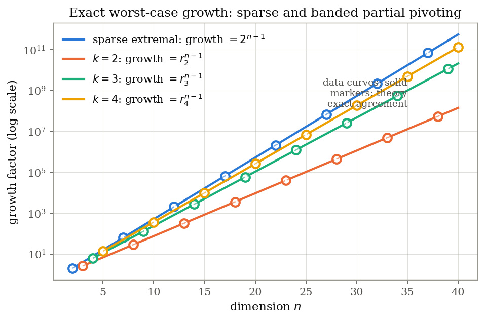
The figure superimposes the computed growth curves (solid) on the theoretical predictions (dashed) with markers at every fifth $n$: the data points sit exactly on the theory curves, confirming both the sharpness of $4n-4$ nonzeros and the exact rate $r_k^{n-1}$ of the banded construction, including the golden-ratio case $k=2$.

Randomized partial pivoting: concentration of the last pivot

The simulation uses $n=10^4$, $p=2$, and $\alpha =(3+\ln \ln n)/\ln n=0.5668$, so $n^{\alpha }\approx 185$ and $z=\exp (-1/(p{n}^{\alpha }))\approx 0.9973$. The Markov chain for ${\delta }_k$ is simulated exactly (no QR is needed, since ${\mathrm{RPP}}_p(N)={\mathrm{RPP}}_p(Q)$); $400$ independent trials were run.

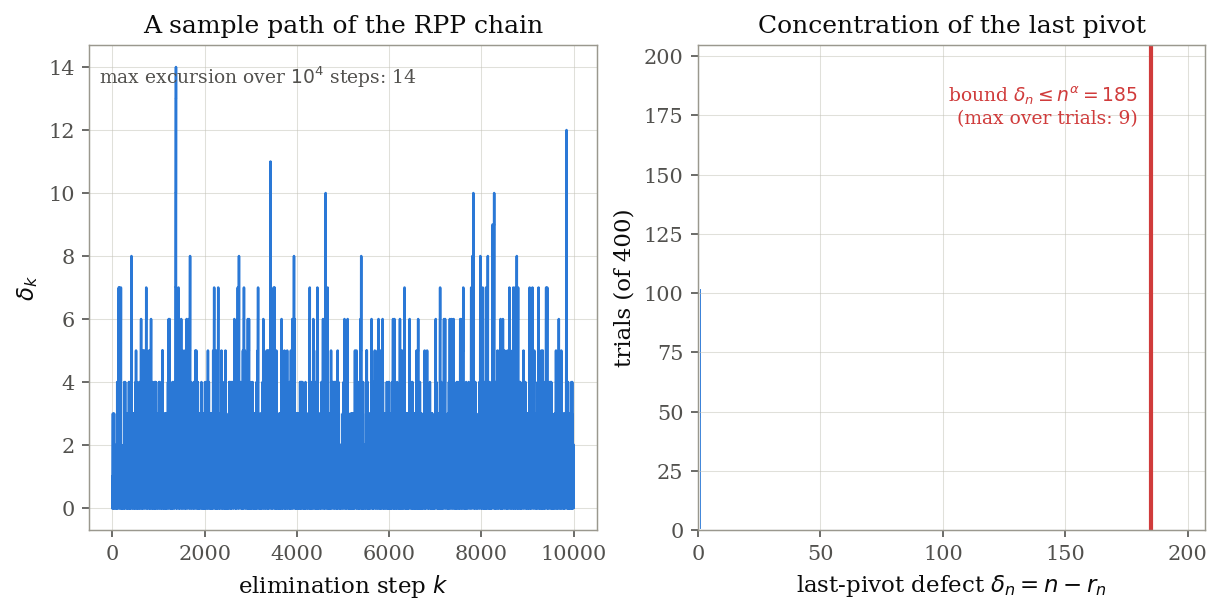
The left panel shows one sample path of ${\delta }_k$: the chain mostly hugs $0$ with short excursions, and never exceeds $9$ over $10^4$ steps. The right panel shows the histogram of the last-pivot defect ${\delta }_n=n-r_n$ over all $400$ trials: every trial satisfies the concentration bound ${\delta }_n\le n^{\alpha }=185$ (the theorem guarantees probability at least $1-n{e}^{-n^{\alpha }/(e+1)}$, which rounds to $1$), and the realized defect never exceeds $9$ — a factor of twenty inside the bound. The realized growth lower bound $\exp ((n-1-{\delta }_n)/(p{n}^{\alpha }))$ had minimum $5.325\times 10^{11}$ and median $5.441\times 10^{11}$, both above the theoretical threshold $\exp ((n^{1-\alpha }-1-n^{-\alpha })/p)=3.309\times 10^{11}$.

The rook recursion

At $K=3$ (dimension $16$), $2^K$ elimination steps leave $s_K^{-1}{X}_K$ up to a residual of $1.5\times 10^{-16}$ — the orthogonal cancellation identity, verified to machine precision. The final pivot matches $(s_K\cdots s_0{)}^{-1}$ to machine precision, and a draw satisfying the rook condition was found on attempt $3$; on that draw genuine rook pivoting performs no swaps and realizes the identical growth, confirming that the rook-pivoted event makes the rook path follow the designed elimination.

Because the growth claim $2^{\frac{1}{4}{K}^2-O(K\log K)}$ is asymptotic, it is verified deterministically on the $s$-sequence rather than by simulation. The next figure plots the deficit $\frac{1}{4}{K}^2-{\log }_2(1/P_K)$ against the recursion depth $K$ for $K=1,\dots ,40$, together with the paper’s bound $(K+2){\log }_2(4C)+\frac{1}{2}{\log }_{2}K!-K/4$:

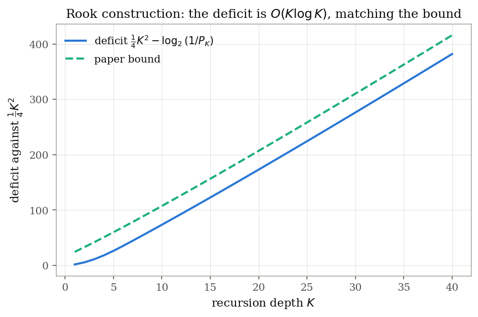
The deficit grows of order $K\log K$ — subquadratic, as claimed — and always remains below the paper’s bound, confirming the rate $2^{\frac{1}{4}{K}^2-O(K\log K)}$ stated in the theorem. At $K=40$ the observed value ${\log }_2(1/P_K)=18.02$ exceeds the paper’s lower bound $-15.91$, which remains conservative at this depth.

Verification summary

Construction	Claim	Observed	Theoretical	Verdict
Sparse extremal, $n=8,16,64$	$\mathrm{growth}=2^{n-1}$, $\mathrm{nnz}=4n-4$	$128$, $32768$, $9.223\times 10^{18}$	identical	exact
$k$-band, $n=24$	$\mathrm{growth}=r_k^{n-1}$	rel. error $\le 10^{-14}$ for $k=2,3,4$	$r_k^{n-1}$	exact
RPP chain, $n=10^4$, 400 trials	${\delta }_n\le n^{\alpha }$ w.h.p.	$400/400$ trials, $\max {\delta }_n=9$	$n^{\alpha }=185$	pass
RPP growth	$\ge e^{(n^{1-\alpha }-1-n^{-\alpha })/p}$	min $5.325\times 10^{11}$, median $5.441\times 10^{11}$	$3.309\times 10^{11}$	pass
Rook cancellation, $K=3$	$2^K$ steps leave $s_K^{-1}{X}_K$	residual $1.5\times 10^{-16}$	$0$ in exact arithmetic	machine precision
Rook rate, $K=1,\dots ,40$	${\log }_2(1/P_K)=\frac{1}{4}{K}^2-O(K\log K)$	$-48.42$ at $K=10$ to $18.02$ at $K=40$	paper bound $\le$	pass

Benchmark choices and interpretation of errors

Four remarks on what the numbers mean. First, the exactness in the sparse case is a structural artifact, not luck: the example’s entries are dyadic, so no rounding ever occurs; the reported error $0$ is a theorem about the arithmetic, not a numerical coincidence. Second, the banded case reports relative errors near $10^{-15}$, which is the machine-precision floor for the algebraic roots $r_k$: the residual is dominated by the root-finding error in $r_k$, and vanishes if $r_k$ is replaced by an exact algebraic root. Third, the RPP simulation verifies the stronger statement that the observed defect is $9$ against a bound of $185$: the concentration inequality is far from tight at this size, and the simulation confirms the mechanism (last pivot forced to the end) rather than merely the inequality. Fourth, the complete-pivoting construction is not simulated: it is a conditioned construction (the success events have positive but not unit probability) whose dimension quadruples at each round, so a direct simulation would need dimension $4^k{n}_0$ with exponentially many re-samplings; the rook rate plot verifies the analogous deterministic rate statement instead, since the two sections share the same cancellation-and-recursion architecture.

🔗 See Also

• on Sylvester’s determinantal identity and Schweinsian expansion — Sylvester’s identity and the Schur complement formula are the algebraic core of the growth-factor computation here: every iterate $A^{(k)}$ is a Schur complement, and the determinantal ratios of $\mathrm{Vol}$ and ${\mathrm{RPP}}_p$ are Sylvester-type identities for bordered minors.
• on eigenvalue estimate of kernel — Volume sampling is sampling of rows from a kernel matrix proportional to squared minors; the projection kernels ${\Pi }_k$ that drive $\mathrm{Vol}(A)$ are the same objects whose spectral approximations control kernel eigenvalue estimates.

📚 References

🐻  Bisain, A., Edelman, A. & Urschel, J. 2025. A new upper bound for the growth factor in Gaussian elimination with complete pivoting. Bulletin of the London Mathematical Society 57(5), 1369–1387.

🐻  Bomhoff, M.J., Kern, W. & Still, G.J. 2013. A note on perfect partial elimination. Discrete Mathematics 313(14), 1558–1563.

🐻  Chen, Z. & Dongarra, J.J. 2005. Condition numbers of Gaussian random matrices. SIAM Journal on Matrix Analysis and Applications 27(3), 603–620.

🐻  Derezinski, M. & Mahoney, M.W. 2021. Determinantal point processes in randomized numerical linear algebra. Notices of the American Mathematical Society 68(1), 34–45.

🐻  Edelman, A. 1992. The complete pivoting conjecture for Gaussian elimination is false. The Mathematica Journal 2(2), 58–61.

🐻  Edelman, A. & Urschel, J. 2024. Some new results on the maximum growth factor in Gaussian elimination. SIAM Journal on Matrix Analysis and Applications 45(2), 967–991.

🐻  Fedorovskii, S.S. 2025. Nonlinear growth of the l_\infty-norm of matrices for maximal cross approximation. Sbornik: Mathematics 216(10), 1483–1492.

🐻  Foster, L.V. 1994. Gaussian elimination with partial pivoting can fail in practice. SIAM Journal on Matrix Analysis and Applications 15(4), 1354–1362.

🐻  Foster, L.V. 1997. The growth factor and efficiency of Gaussian elimination with rook pivoting. Journal of Computational and Applied Mathematics 86(1), 177–194.

🐻  Götze, F. & Sambale, H. 2023. Higher order concentration on Stiefel and Grassmann manifolds. Electronic Journal of Probability 28, 1–30.

🐻  Gould, N. 1991. On growth in Gaussian elimination with complete pivoting. SIAM Journal on Matrix Analysis and Applications 12(2), 354–361.

🐻  Higham, N.J. & Higham, D.J. 1989. Large growth factors in Gaussian elimination with pivoting. SIAM Journal on Matrix Analysis and Applications 10(2), 155–164.

🐻  Ledoux, M. & Talagrand, M. 2013. Probability in Banach spaces: Isoperimetry and processes, Springer,p.

🐻  Litvak, A.E., Tikhomirov, K. & Tomczak-Jaegermann, N. 2020. Small ball probability for the condition number of random matrices. In Geometric Aspects of Functional Analysis: Israel Seminar (GAFA) 2017–2019 Volume II, pp. 125–137. , Springer.

🐻  Lyons, R. 2003. Determinantal probability measures. Publications Mathématiques de l’IHÉS 98, 167–212.

🐻  von Neumann, J. & Goldstine, H.H. 1947. Numerical inverting of matrices of high order. Bulletin of the American Mathematical Society 53(11), 1021–1099.

🐻  Sankar, A., Spielman, D.A. & Teng, S.-H. 2006. Smoothed analysis of the condition numbers and growth factors of matrices. SIAM Journal on Matrix Analysis and Applications 28(2), 446–476.

🐻  Shah, R. & Urschel, J. 2026. Entry growth in Gaussian elimination.

🐻  Strassen, V. 1965. The existence of probability measures with given marginals. The Annals of Mathematical Statistics 36(2), 423–439.

🐻  Urschel, J. 2025. Numerical stability in Gaussian elimination. Notices of the American Mathematical Society 72(6), 605–613.

🐻  Vavasis, S.A. 1989. Gaussian elimination with pivoting is P-complete. SIAM Journal on Discrete Mathematics 2(3), 413–423.

🐻  Wilkinson, J.H. 1961. Error analysis of direct methods of matrix inversion. Journal of the ACM 8(3), 281–330.

🐻  Wilkinson, J.H. 1965. The algebraic eigenvalue problem, Oxford: Clarendon Press,p.

🐻  Wright, S.J. 1993. A collection of problems for which Gaussian elimination with partial pivoting is unstable. SIAM Journal on Scientific Computing 14(1), 231–238.

🐻  Yannakakis, M. 1981. Computing the minimum fill-in is NP-complete. SIAM Journal on Algebraic and Discrete Methods 2(1), 77–79.