Komlós discrepancy from signs to complex phases

Overview

Can vectors of Euclidean norm at most one always be assigned signs so that every coordinate of their sum stays bounded by an absolute constant? The Komlós conjecture asks for a bound independent of both the dimension and the number of vectors. Guo, Fang, and Lu prove a bound of $3\sqrt{2\pi }$ using directional total variation and a convex-body transform (Guo, Fang & Lu, 2026). Karingula and Lovett simplify the argument to obtain the constant $36$ using finite probability distributions and elementary calculus (Karingula & Lovett, 2026).

These two proofs turn overlap between translated distributions into freedom to choose signs. An extra coordinate preserves that freedom: a bit in the elementary proof, and a continuous height in the analytic proof. Guillen and Kobzar study a relaxation allowing unit complex phases and prove a constant bound through a Bellman-function minimum principle (Guillen & Kobzar, 2026). Their proof uses the two real coordinates of each phase to find a feasible direction of negative curvature.

The versions discussed are Karingula–Lovett, arXiv:2609.20979v2, revised September 22, 2026; Guo–Fang–Lu, arXiv:2609.11189v1, submitted September 10, 2026; and Guillen–Kobzar, arXiv:2609.15071v2, revised September 21, 2026. The elementary proof is given in full, followed by the main analytic and variational mechanisms of the other two papers.

🏷️ Discrepancy and the Komlós problem

Let $A\in {\mathbb{R}}^{d\times n}$ have columns $v_1,\dots ,v_n$. A signing is a vector $\epsilon \in \{-1,1{\}}^n$. Its discrepancy is the largest absolute coordinate of

$$A\epsilon =\sum _{i=1}^n{\epsilon }_i{v}_i.$$

The discrepancy of the matrix is

$$\mathrm{disc}(A)=\underset{\epsilon \in \{-1,1{\}}^n}{\min }\Vert A\epsilon {\Vert }_{\infty }.$$

Here $\Vert x{\Vert }_2=({\sum }_j{x}_j^2{)}^{1/2}$ and $\Vert x{\Vert }_{\infty }={\max }_j|x_j|$. The Komlós hypothesis is a bound on each column:

$$\Vert v_i{\Vert }_2^2=\sum _{j=1}^d{A}_{ji}^2\le 1.$$

There is no bound on a row’s squared norm, and $n$ and $d$ are arbitrary.

The two signing bounds

For every finite family $v_1,\dots ,v_n\in {\mathbb{R}}^d$ with $\Vert v_i{\Vert }_2\le 1$, there is a signing satisfying

$${\Vert \sum _i{\epsilon }_i{v}_i\Vert }_{\infty }<3\sqrt{2\pi }$$

by Guo–Fang–Lu, Theorem 1.1. Karingula–Lovett, Theorem 1.2, gives an elementary proof of

$${\Vert \sum _i{\epsilon }_i{v}_i\Vert }_{\infty }\le 36.$$

These are existence statements for real scalar signs and the final sum. The first constant is approximately $7.52$; neither paper asserts that its constant is optimal.

The problem also describes simultaneous rounding. If $x=(1+\epsilon )/2\in \{0,1{\}}^n$, then

$$A\left(x-\frac{1}{2}1\right)=\frac{1}{2}A\epsilon .$$

Thus one can round all the half-integer choices while keeping every linear constraint within a constant error under the column normalization.

Independent random signs do not by themselves give this conclusion. For a fixed row $j$,

$$\mathbb{E}{\left(\sum _i{\epsilon }_i{A}_{ji}\right)}^2=\sum _i{A}_{ji}^2,$$

which may equal $n$. If all columns are the first coordinate vector, a random signing has root-mean-square discrepancy $\sqrt{n}$, although choosing nearly equal numbers of positive and negative signs gives discrepancy at most one. The task is to arrange cancellation across all rows simultaneously.

Complex phases and rank-two vector discrepancy

Write $\mathbb{T}=\{z\in \mathbb{C}:|z|=1\}$. For a complex matrix $M\in {\mathbb{C}}^{d\times n}$, define

$$\mathrm{cdisc}(M)=\underset{z\in {\mathbb{T}}^n}{\min }\Vert Mz{\Vert }_{\infty },$$

where the norm takes the largest complex modulus. For a real matrix $A$, identify $z_j=e^{i{\theta }_j}$ with $u_j=(\cos {\theta }_j,\sin {\theta }_j)\in {\mathbb{R}}^2$. Then

$$\begin{array}{rl}\mathrm{cdisc}(A)& ={\mathrm{Vdisc}}_2(A)\\ & =\underset{u_j\in {\mathbb{S}}^1}{\min }\underset{i}{\max }{\Vert \sum _j{A}_{ij}{u}_j\Vert }_2.\end{array}$$

This is rank-two vector discrepancy. Boolean signs are the special choices $u_j=(\pm 1,0)$, so $\mathrm{cdisc}(A)\le \mathrm{disc}(A)$. An arbitrary phase assignment need not yield a comparably good Boolean assignment by rounding each phase. Guillen–Kobzar prove the phase bound by a separate variational argument, developed below.

🏷️ Translation overlap and convex combinations

For a finitely supported probability distribution $P$ on ${\mathbb{R}}^d$, write

$$\begin{array}{rl}\mu (P)& =\sum _{x}P(x)x,\\ \mathrm{supp}(P)& =\{x:P(x)>0\}.\end{array}$$

The convex hull of a set consists of its finite weighted averages with nonnegative weights summing to one. In particular, $\mu (P)\in \mathrm{conv}(\mathrm{supp}P)$.

The translate $P+u$ is the law of $X+u$ when $X$ has law $P$; its mass at $x$ is $P(x-u)$. Define the shift distance

$$\begin{array}{c}\Delta (P,u)=d_{\mathrm{TV}}(P,P+u)\\ =\frac{1}{2}\sum _x|P(x)-P(x-u)|.\end{array}$$

The identity $\min (a,b)=(a+b-|a-b|)/2$ gives

$$\begin{array}{c}\sum _x\min \{P(x),P(x-u)\}\\ =1-\Delta (P,u).\end{array}$$

This is a mass-overlap statement: when the shift distance is at most $1/3$, at least $2/3$ of the mass can be matched between the two distributions. For continuous densities the same formulas hold with integrals in place of sums.

A distribution in a cube can have substantial overlap with all the translations of interest even though the cube has tiny Gaussian measure. Choosing the distribution matters. For example, let $U$ be uniform on $[-a,a{]}^d$. Directly computing the intersection of two cubes gives

$$\Delta (U,u)=1-\prod _{j=1}^d{\left(1-\frac{|u_j|}{2a}\right)}_{+},$$

where $r_{+}=\max (r,0)$. Along the unit diagonal $e=(1,\dots ,1)/\sqrt{d}$,

$$\underset{h\downarrow 0}{\lim }\frac{\Delta (U,he)}{h}=\frac{\sqrt{d}}{2a}.$$

The sharp boundary of the uniform density therefore introduces dimension dependence. The proofs use densities that taper to zero at the boundary, together with an invariant that survives the signing procedure.

🏷️ The elementary balancing principle

The central discrete statement has no norm restriction on the vectors. Its hypothesis concerns their translations instead.

Near invariance implies a signed displacement

Let $P$ be a finitely supported probability distribution on ${\mathbb{R}}^d$. If

$$\Delta (P,6v_i)\le \frac{1}{3}(1\le i\le n),$$

then some signs satisfy

$$\begin{array}{c}\mu (P)+\sum _i{\epsilon }_i{v}_i\\ \in \mathrm{conv}(\mathrm{supp}P).\end{array}$$

This is Karingula–Lovett, Lemma 1.4. Allowing an arbitrary mean is essential because the proof adds a coordinate whose mean is positive. (Karingula & Lovett, 2026)

The proof uses induction on the number of vectors, simultaneously in every dimension. It splits the distribution, applies induction in one extra dimension, and then moves a suitable convex combination back to the original support.

Splitting into two levels

For a vector $w$, define a nonnegative function on ${\mathbb{R}}^d\times \{0,1\}$ by

$$\begin{array}{c}(T_{w}P)(x,0)=\frac{1}{2}\max \{p_{+},p_{-}\},\\ (T_{w}P)(x,1)=\frac{1}{2}\min \{p_{+},p_{-}\},\\ p_{\pm }=P(x\pm w).\end{array}$$

It is zero at other values of the last coordinate. The possible parents of $(x,b)$ are $x+w$ and $x-w$. A parent is available when it belongs to $\mathrm{supp}P$. Every positive-mass state has at least one available parent; every state with bit $b=1$ has both.

Adding the maximum and minimum shows that $T_w$ preserves total mass, including for nonnegative inputs of mass less than one. The opposite shifts cancel in the first $d$ coordinates of the mean. Consequently, if $Q=T_{w}P$, then

$$\begin{array}{rl}\mu (Q)& =(\mu (P),\beta ),\\ \beta =\underset{Q}{\mathrm{Pr}}[b=1]& =\frac{1-\Delta (P,2w)}{2}.\end{array}$$

The factor $2w$ occurs because the two possible parents are separated by that vector.

Shift distances cannot increase

Write $\bar{u}=(u,0)$. The splitting map satisfies

$$\Delta (T_{w}P,\bar{u})\le \Delta (P,u).$$

Here is a proof that also explains why sorting the two masses is useful. Put

$$H(x)=\min \{P(x),P(x-u)\}.$$

Both minimum and maximum preserve pointwise inequalities, so $T_w$ is monotone. It also commutes with horizontal translations. Since $H\le P$ and $H\le P+u$,

$$T_{w}H\le \min \{T_{w}P,T_{w}P+\bar{u}\}.$$

The left side has mass ${\sum }_{x}H(x)=1-\Delta (P,u)$. The right side is the common mass after splitting. This proves contraction. The map $T_w$ need not be linear; monotonicity, mass preservation, and translation compatibility suffice.

The extra bit survives induction

Let $v=v_n$ and take $Q=T_{3v}P$. The hypothesis at $6v$ gives

$$\beta =\frac{1-\Delta (P,6v)}{2}\ge \frac{1}{3}.$$

Extend the remaining vectors to ${\bar{v}}_i=(v_i,0)$. Shift contraction preserves their hypotheses. Induction therefore gives signs for $i<n$ such that

$$\begin{array}{c}(\mu (P)+s,\beta )\in \mathrm{conv}(\mathrm{supp}Q),\\ s=\sum _{i<n}{\epsilon }_i{v}_i.\end{array}$$

Choose a distribution $R$ supported on $\mathrm{supp}Q$ with this mean. It may assign very different masses from $Q$. Nevertheless,

$$\underset{R}{\mathrm{Pr}}[b=1]={\mathbb{E}}_{R}b=\beta .$$

The bit turns a lower bound on usable mass into a linear constraint on every convex combination produced by induction. Merely remembering that some points have two parents would lose this quantitative information.

An exact correction of the mean

Move each state $(x,0)$ of $R$ to any available parent $x\pm 3v$. These moves change the first $d$ coordinates of the mean by $av$, where

$$|a|\le 3(1-\beta )\le 2.$$

For each state $(x,1)$, both parents are available. Send a common fraction $t$ of its mass to $x+3v$ and the remaining fraction to $x-3v$. The aggregate contribution is

$$3\beta (2t-1)v.$$

As $t$ ranges over $[0,1]$, its scalar coefficient fills $[-3\beta ,3\beta ]$, which contains $[-1,1]$. Choose ${\epsilon }_n$ with the sign of $a$, taking ${\epsilon }_n=1$ when $a=0$. Because $|a|\le 2$,

$$|{\epsilon }_n-a|\le 1\le 3\beta .$$

The explicit choice

$$t=\frac{1}{2}+\frac{{\epsilon }_n-a}{6\beta }$$

lies in $[0,1]$ and makes the total displacement exactly ${\epsilon }_{n}v$.

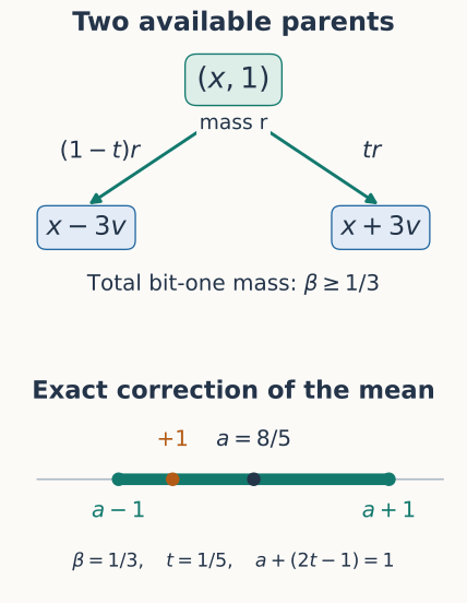
The bit-one mass can move to either parent. In the scalar example below the schematic, $\beta =1/3$ and $a=8/5$: the available correction interval reaches the target $+1$, using $t=1/5$.

All the moved mass lies on $\mathrm{supp}P$, so its mean lies in that convex hull. Its mean is precisely

$$\mu (P)+s+{\epsilon }_{n}v.$$

This closes the induction. The initial case $n=0$ is the definition of the mean as a convex combination. Zero vectors cause no difficulty: their signing has no effect.

Notice that the transported masses need not be bounded by the original values $P(x)$. The conclusion requires a distribution on the same support, not a redistribution obeying capacities at each point. This freedom is part of the convex-hull argument.

🏷️ A cube density with dimension-free overlap

It remains to construct the distribution required by the balancing principle. The continuous construction is particularly simple after taking a square root.

Define

$$\begin{array}{c}b(t)=\frac{(6-|t|{)}_{+}}{12},\\ f(x)=\prod _{j=1}^{d}b(x_j),\\ F(x)=f(x{)}^2.\end{array}$$

Direct one-dimensional integration gives

$$\begin{array}{c}\int b^2=1,\int b{b}^{\prime }=0,\\ \int (b^{\prime }{)}^2=\frac{1}{12}.\end{array}$$

For instance, $\int b^2=2{\int }_0^6(6-t{)}^2/144dt=1$. Thus $F$ is a probability density supported on $[-6,6{]}^d$. It is even, so its mean is zero.

For a vector $u$, expand the square of the directional derivative ${\partial }_{u}f=u\cdot \nabla f$. Each diagonal term contributes $u_j^2/12$. Every mixed term contains a factor $\int b{b}^{\prime }=0$. Hence

$$\Vert {\partial }_{u}f{\Vert }_{L^2}^2=\frac{\Vert u{\Vert }_2^2}{12}.$$

This orthogonality is where the Euclidean norm enters. Bounding coordinate derivatives separately by a triangle inequality would instead introduce $\Vert u{\Vert }_1$.

The fundamental theorem of calculus along a segment gives, almost everywhere,

$$\begin{array}{c}f(x+u)-f(x)\\ ={\int }_0^1{\partial }_{u}f(x+tu)dt.\end{array}$$

Cauchy–Schwarz in $t$, followed by integration in $x$, yields

$$\begin{array}{rl}\Vert f(\cdot +u)-f{\Vert }_{L^2}& \le \Vert {\partial }_{u}f{\Vert }_{L^2}\\ & =\frac{\Vert u{\Vert }_2}{\sqrt{12}}.\end{array}$$

The finitely many corners of the tent function do not affect these integrals. Factoring a difference of squares and using $\Vert f{\Vert }_{L^2}=1$ now gives

$$\begin{array}{c}\Delta (F,u)=\frac{1}{2}\Vert f(\cdot +u{)}^2-f^2{\Vert }_{L^1}\\ \le \frac{1}{2}\Vert f(\cdot +u)-f{\Vert }_{L^2}\\ \cdot \Vert f(\cdot +u)+f{\Vert }_{L^2}\\ \le \frac{\Vert u{\Vert }_2}{\sqrt{12}}.\end{array}$$

Thus every unit Euclidean translation has shift distance at most $1/\sqrt{12}<1/3$, in every dimension. This is Karingula–Lovett, Lemma 4.1. (Karingula & Lovett, 2026)

Discretization on a compatible grid

Suppose first that all $v_i$ have rational coordinates. Choose a positive integer $N$ with $N{v}_i\in {\mathbb{Z}}^d$ for every $i$, and round a sample from $F$ to the nearest point of

$$G=N^{-1}{\mathbb{Z}}^d.$$

Equivalently, with $C_N=[-1/(2N),1/(2N){)}^d$, set

$$P(x)={\int }_{C_N}F(x+z)dz,$$

for $x\in G$, and put $P=0$ off the grid. Because $\pm 6$ are grid points, rounding keeps the support in $[-6,6{]}^d$. Symmetry gives $P(-x)=P(x)$ and hence $\mu (P)=0$; the cell boundaries have probability zero.

For any $u\in G$, rounding commutes with translation by $u$. Set $h_u(z)=F(z-u)-F(z)$. Taking absolute values inside each cell integral gives

$$\begin{array}{c}\Delta (P,u)\\ \le \frac{1}{2}\sum _{x\in G}{\int }_{x+C_N}|h_u(z)|dz\\ =\Delta (F,u)\le \frac{\Vert u{\Vert }_2}{\sqrt{12}}.\end{array}$$

This is the elementary form of contraction of total variation under a measurable map. Compatibility of the grid with every $v_i$ is necessary for the translated rounded law to equal $P+v_i$.

The constant and the passage to real inputs

The discrete distribution satisfies $\Delta (P,v_i)\le 1/3$. Apply the balancing principle to the vectors $v_i/6$. It gives

$$\begin{array}{c}\frac{1}{6}\sum _i{\epsilon }_i{v}_i\in \mathrm{conv}(\mathrm{supp}P),\\ \mathrm{conv}(\mathrm{supp}P)\subseteq [-6,6{]}^d.\end{array}$$

Multiplying by six proves the bound $36$. One factor of six comes from the translation scale in the balancing lemma; the other is the half-side of the cube supporting $P$.

For real inputs, truncate each coordinate toward zero on finer rational grids. This produces rational vectors $v_i^{(m)}\to v_i$ with $\Vert v_i^{(m)}{\Vert }_2\le 1$. There are only $2^n$ sign vectors, so one signing occurs along an infinite subsequence of the rational approximations. Passing to the limit with that fixed signing proves the same non-strict bound for the original vectors.

🏷️ Directional variation and the geometric transform

Guo–Fang–Lu preserve an infinitesimal translation bound while changing the supporting convex set. For a differentiable density $\rho$, its directional variation is

$$V_u(\rho )={\int }_{{\mathbb{R}}^d}|{\partial }_u\rho (x)|dx.$$

To include nonsmooth densities, define it by testing distributional derivatives:

$$V_u(\rho )=\underset{\begin{array}{c}\varphi \in C_c^1({\mathbb{R}}^d)\\ \Vert \varphi {\Vert }_{\infty }\le 1\end{array}}{\sup }\int \rho {\partial }_u\varphi .$$

Here $C_c^1$ denotes continuously differentiable, compactly supported test functions. A function belongs to $BV$ if its distributional gradient is a finite vector measure. Directional variation measures that derivative, including jumps across the boundary of the support.

For example, the zero extension of $\rho =(2a{)}^{-1}{1}_{(-a,a)}$ has $V_1(\rho )=1/a$, although its derivative inside the interval is zero. The two endpoint jumps each contribute $1/(2a)$.

For $BV$ densities,

$$\begin{array}{c}\Vert \rho (\cdot +hu)-\rho {\Vert }_{L^1}\le |h|V_u(\rho ),\\ V_u(\rho )=\underset{h\to 0}{\lim }\frac{\Vert \rho (\cdot +hu)-\rho {\Vert }_{L^1}}{|h|}.\end{array}$$

Thus total variation distance is bounded by $|h|V_u(\rho )/2$. The factor $1/2$ belongs to the distance between probability laws, not to $V_u$.

Let $K$ be a nonempty bounded open convex set. Write $\mathcal{P}(K)$ for the nonnegative $BV$ densities of mass one that vanish almost everywhere outside $K$. Their topological supports may meet $\partial K$. The invariant is the existence of a single $\rho \in \mathcal{P}(K)$ such that

$$V_u(\rho )\le \kappa \Vert u{\Vert }_2(u\in {\mathbb{R}}^d).$$

The open-set Banaszczyk transform

For a vector $v$, define

$$\begin{array}{rl}{\mathcal{T}}_{v}K& =((K-v)\cap (K+v))\\ & +\{tv:-2<t<2\}.\end{array}$$

For $v\ne 0$, inspect a line parallel to $v$. A fiber of length at most $2\Vert v{\Vert }_2$ disappears. A longer fiber is shortened by $\Vert v{\Vert }_2$ at both ends by the intersection, then lengthened by $2\Vert v{\Vert }_2$ at both ends by the addition. Its net expansion is $\Vert v{\Vert }_2$ at each end.

The crucial inclusion is

$${\mathcal{T}}_{v}K\subseteq (K-v)\cup (K+v).$$

Indeed, write $y=z+tv$ with $z-v,z+v\in K$ and $|t|<2$. If $t\ge 0$, then $y-v=z+(t-1)v\in K$ by convexity. If $t\le 0$, then $y+v\in K$.

Finite-step stability

Suppose $K$ is nonempty, bounded, open, and convex, and some $\rho \in \mathcal{P}(K)$ satisfies $V_u(\rho )\le \kappa \Vert u{\Vert }_2$ in every direction. If

$$\kappa \Vert v{\Vert }_2\le \frac{1}{3},$$

then ${\mathcal{T}}_{v}K$ is nonempty and supports a new probability density with the same directional bound $\kappa$. This is Guo–Fang–Lu, Proposition 2.2. (Guo, Fang & Lu, 2026)

The density may change at every step, but its numerical bound does not grow. Starting with a centrally symmetric $K_0$, form $K_j={\mathcal{T}}_{v_j}{K}_{j-1}$. Stability keeps all these sets nonempty, and the transform preserves convexity and central symmetry. Therefore $0\in K_n$.

Starting from $z_n=0$, use the inclusion to choose signs backwards so that

$$z_{j-1}=z_j+{\epsilon }_j{v}_j\in K_{j-1}.$$

Then $z_0={\sum }_j{\epsilon }_j{v}_j\in K_0$. Symmetry is needed for the final starting point $0\in K_n$; it is not a hypothesis of finite-step stability itself.

🏷️ The sharper cube constant

For $C>0$, consider the cosine-squared product density, defined inside $(-C,C{)}^d$ by

$${\rho }_C(x)=C^{-d}\prod _{j=1}^d{\cos }^2\left(\frac{\pi x_j}{2C}\right).$$

Set ${\rho }_C=0$ outside the cube. Each factor integrates to one after normalization and vanishes at the endpoints, so extending by zero creates no boundary jump. Its square root is the normalized first Dirichlet eigenfunction of the cube.

If $X$ has this density and $T_j=\tan (\pi X_j/(2C))$, differentiation gives

$$V_u({\rho }_C)=\frac{\pi }{C}\mathbb{E}\left|\sum _j{u}_j{T}_j\right|.$$

The $T_j$ are independent with density $2/[\pi (1+t^2{)}^2]$. They have the representation

$$T_j\stackrel{\mathrm{law}}{=}\frac{G_j}{\sqrt{S_j}},$$

where all variables are independent, $G_j$ is a standard real Gaussian, and $S_j$ has the ${\chi }^2$ distribution with three degrees of freedom. The latter means the sum of squares of three independent standard Gaussians; its reciprocal has expectation one.

Condition on the $S_j$. The sum is a centered Gaussian of variance ${\sum }_j{u}_j^2/S_j$, so

$$\begin{array}{rl}\mathbb{E}\left|\sum _j{u}_j{T}_j\right|& =\sqrt{\frac{2}{\pi }}\mathbb{E}\sqrt{\sum _j\frac{u_j^2}{S_j}}\\ & \le \sqrt{\frac{2}{\pi }}\Vert u{\Vert }_2.\end{array}$$

The inequality is Jensen’s inequality for the square root. Consequently,

$$V_u({\rho }_C)\le \frac{\sqrt{2\pi }}{C}\Vert u{\Vert }_2.$$

Taking $C=3\sqrt{2\pi }$ makes $\kappa =1/3$, so every input vector of norm at most one meets the stability condition. The backward signing ends inside the open cube $(-C,C{)}^d$, giving the strict discrepancy bound. This is the argument of Lemma 2.4 and Theorem 1.1. (Guo, Fang & Lu, 2026)

Using Cauchy–Schwarz directly on the $T_j$ would give $\pi /C$ instead of $\sqrt{2\pi }/C$. The Gaussian-mixture representation accounts for the improvement in the stated constant.

🏷️ Lifting overlap into a prescribed section

Finite-step stability is the substantive analytic theorem. Its proof has two ingredients: a lift with enough average height, and a variational principle transferring horizontal variation bounds to one specified height.

The lift and its rearrangement

Given $K$, $v$, and a density $\rho$ on $K$, set

$$\begin{array}{c}B=\{(y,s):|s|<3,y+sv\in K\},\\ R(y,s)=\frac{1}{6}\rho (y+sv)1_{\{|s|<3\}}.\end{array}$$

The density $R$ has mass one and is supported in $B$. A horizontal translation acts only on $y$, giving

$$V_{(u,0)}(R)=V_u(\rho ).$$

Each vertical fiber of $B$ is an interval. Replace it by a centered interval of the same length $\ell (y)$ to obtain the Steiner symmetral

$$B^{\star }=\{(y,s):|s|<\ell (y)/2\}.$$

Convexity of $B$ makes $B^{\star }$ convex. Its height-one section is exactly

$$\begin{array}{rl}\{y:(y,1)\in B^{\star }\}& =\{y:\ell (y)>2\}\\ & ={\mathcal{T}}_{v}K.\end{array}$$

To see the last equality, an open interval inside $(-3,3)$ has length greater than two precisely when it contains $c-1,c+1$ for some $|c|<2$. These two heights say that $y+cv-v$ and $y+cv+v$ lie in $K$.

Rearrange the density on each vertical fiber symmetrically and decreasingly, obtaining $R^{\star }$. This preserves mass and support in $B^{\star }$. It also contracts the $L^1$ distance between any pair of fibers: at each level, centered intervals have the largest possible overlap among sets of the prescribed lengths. Integrating the level sets gives

$$V_{(u,0)}(R^{\star })\le V_u(\rho ).$$

The sorting in the discrete splitting operator is a two-level counterpart of this rearrangement.

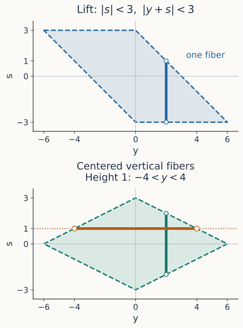
For $K=(-3,3)$ and $v=1$, the lift is a parallelogram. Centering its vertical fibers gives a diamond whose height-one section is $(-4,4)={\mathcal{T}}_{1}K$. Boundaries are excluded. For the uniform input density on $K$, the rearranged mean absolute height is exactly one.

The exact height identity

Rearrangement can lower the mean absolute height. Its loss is determined by translation overlap:

$$\begin{array}{c}\int |s|R^{\star }(y,s)dyds\\ =\frac{3}{2}-\frac{1}{24}{\int }_0^6(6-h)\\ \cdot \Vert \rho -\rho (\cdot +hv){\Vert }_{L^1}dh.\end{array}$$

For the normalization, a centered interval of length $\ell$ has first absolute moment ${\ell }^2/4$. Applying this to all superlevel sets of each rearranged fiber expresses the moment as an integral over two original heights $r,s\in (-3,3)$. Integrating in $y$ produces the overlap

$$O(h)=1-\frac{1}{2}\Vert \rho -\rho (\cdot +hv){\Vert }_{L^1}.$$

Pairs of heights separated by $h$ have weight $2(6-h)$. The resulting moment is $\frac{1}{12}{\int }_0^6(6-h)O(h)dh$, which gives the displayed identity.

Since $\Vert \rho -\rho (\cdot +hv){\Vert }_1\le h{V}_v(\rho )$ and ${\int }_0^{6}h(6-h)dh=36$,

$$\int |s|R^{\star }\ge \frac{3}{2}-\frac{3}{2}{V}_v(\rho )\ge 1.$$

The last inequality uses $V_v(\rho )\le \kappa \Vert v{\Vert }_2\le 1/3$. Thus the rearranged density retains enough average height to reach the section encoding sign recovery.

A common density on the prescribed section

Let $D_t=\{y:(y,t)\in B^{\star }\}$ for $t\ge 0$. Symmetry and convexity make these sections nested:

$$D_t\subseteq D_s(0\le s\le t),$$

whenever they are nonempty. They also satisfy

$$(1-\theta )D_s+\theta D_t\subseteq D_{(1-\theta )s+\theta t}.$$

To handle all directional bounds together, fix unit vectors $u_1,\dots ,u_N$ and weights ${\alpha }_{\ell }\ge 0$ with ${\sum }_{\ell }{\alpha }_{\ell }=1$. Define

$$\begin{array}{rl}H(\xi )& =\sum _{\ell }{\alpha }_{\ell }|u_{\ell }\cdot \xi |,\\ E_H(\rho )& =\sum _{\ell }{\alpha }_{\ell }{V}_{u_{\ell }}(\rho ),\\ h_H(D)& =\underset{\rho \in \mathcal{P}(D)}{\inf }{E}_H(\rho ).\end{array}$$

The last quantity is an anisotropic Cheeger value. For a smooth set $E\subset D$, the energy of the uniform density on $E$ is its boundary cost divided by its volume:

$$E_H\left(\frac{1_E}{|E|}\right)=\frac{1}{|E|}{\int }_{\partial E}H({\nu }_E)dS.$$

Here ${\nu }_E$ is the unit normal. The coarea formula extends this interpretation to general densities by integrating their superlevel sets.

Convexity of the Cheeger value

For nonempty bounded open convex sets $D_0,D_1$,

$$\begin{array}{c}{h}_H((1-\theta )D_0+\theta D_1)\\ \le (1-\theta )h_H(D_0)+\theta h_H(D_1).\end{array}$$

This holds even when $H$ vanishes in some nonzero directions. It is Guo–Fang–Lu, Lemma 3.2.

Proof outline: eigenvalue convexity and the limit as $p$ tends to one

The variational input comes from first Dirichlet eigenvalues. Let $H$ be a norm smooth away from zero, with $D^2(H^2)$ positive definite there. For $p>1$, define

$$\begin{array}{c}{\lambda }_{p,H}(D)\\ =\underset{0\ne f\in W_0^{1,p}(D)}{\inf }\frac{{\int }_{D}H(\nabla f{)}^p}{{\int }_D|f{|}^p}.\end{array}$$

The space $W_0^{1,p}(D)$ is the closure of smooth, compactly supported functions in the norm controlling the function and its first derivatives in $L^p$. An eigenvalue convexity theorem gives the same Minkowski inequality for ${\lambda }_{p,H}$, and

$$\underset{p\downarrow 1}{\lim }{\lambda }_{p,H}(D)=h_H(D).$$

For the lower bound in this limit, insert $|f{|}^p/\int |f{|}^p$ into the Cheeger variational problem and use Hölder:

$$h_H(D)\le p{\left(\frac{\int H(\nabla f{)}^p}{\int |f{|}^p}\right)}^{1/p}.$$

For the upper bound, use a fixed smooth density nearly minimizing $h_H(D)$ as a Rayleigh test and let $p\downarrow 1$. Such smooth densities approximate the global $BV$ class by first contracting support into the convex domain, then mollifying.

Guo–Fang–Lu’s appendix develops the eigenvalue argument using log-concavity of first eigenfunctions and infimal convolution of their negative logarithms. The Hessian comparison is an arithmetic–harmonic inequality for positive matrices; a cutoff handles points where the gradient vanishes. This is the deeper analytic input. To reach a possibly degenerate $H$, they use

$$\begin{array}{c}{H}_{ϵ}(\xi )\\ =\sum _{\ell }{\alpha }_{\ell }\sqrt{(u_{\ell }\cdot \xi {)}^2+{ϵ}^2\Vert \xi {\Vert }_2^2}\end{array}$$

and pass to the limit in the variational infima. This avoids assuming uniform regularity of minimizing densities as $H_{ϵ}$ degenerates. (Guo, Fang & Lu, 2026)

Domain monotonicity and Cheeger convexity imply that $g(t)=h_H(D_t)$ is nondecreasing and convex. Let

$$\begin{array}{c}q(s)=\int R^{\star }(y,s)dy,\\ M=\int |s|q(s)ds.\end{array}$$

The normalized slice at height $s$ has energy divided by $q(s)$, so slicing the horizontal variation estimate yields

$$\int q(s)h_H(D_{|s|})ds\le \kappa .$$

Jensen’s inequality and $M\ge 1$ now give

$$\begin{array}{rl}{h}_H(D_1)& \le h_H(D_M)\\ & \le \int q(s)h_H(D_{|s|})ds\\ & \le \kappa .\end{array}$$

All these sections are nonempty: the height distribution is supported strictly below the finite maximal height, so its mean $M$ is also strictly below that height.

This bounds every weighted combination of variations. Fix a finite list of unit directions containing the coordinate basis. Convex separation shows that the infimum of the maximum of their variations is at most $\kappa$: a strictly larger infimum would produce a nonnegative weighted combination with infimum greater than $\kappa$, contradicting the inequality just proved. A minimizing sequence has uniformly bounded coordinate variations, hence a uniform $BV$ bound. Compactness in $L^1$ and lower semicontinuity of each variation then give a probability density on $D_1$ attaining the finite-list bound.

Now take increasing finite lists containing the coordinate basis and a countable dense set of unit directions. All the corresponding densities have total variation at most $d\kappa$, so another application of compactness gives a single $L^1$ limit. Lower semicontinuity preserves every listed directional bound. Continuity in the direction, followed by homogeneity, gives

$$V_u(\tilde{\rho })\le \kappa \Vert u{\Vert }_2\text{for all }u.$$

Since $D_1={\mathcal{T}}_{v}K$, this proves stability. It is not enough to find a different favorable slice for each direction: the next signing step requires all bounds on the same density. The separation and compactness argument is exactly what enforces that compatibility.

🏷️ Complex phases and the Bellman minimum principle

Guillen–Kobzar obtain a constant bound for phases through a different use of continuous freedom. Each coefficient moves in a two-dimensional disk until it reaches the boundary circle.

Complex and rank-two discrepancy

If $A$ is real and every column has Euclidean norm at most one, then

$$\mathrm{cdisc}(A)={\mathrm{Vdisc}}_2(A)\le 46\sqrt{2}.$$

If $M$ is complex and ${\sum }_i|M_{ij}{|}^2\le 1$ for every column, then

$$\mathrm{cdisc}(M)\le 92\sqrt{2}.$$

These are the bounds of Guillen–Kobzar, Theorem 1.3 and Corollary 1.5. The proof is a variational existence argument. (Guillen & Kobzar, 2026)

The factor two for complex inputs follows by writing $M=A+iB$ and stacking $A$ and $B$ into a real matrix. Its column norms remain at most one. A common phase vector controls both $Az$ and $Bz$, and $\Vert Mz{\Vert }_{\infty }\le \Vert Az{\Vert }_{\infty }+\Vert Bz{\Vert }_{\infty }$.

Fractional phases and the state variables

For the real-matrix theorem, allow coefficients

$$\begin{array}{c}x=(x_1,\dots ,x_n),\\ x_j\in {\overline{B}}_2\subset {\mathbb{R}}^2,\end{array}$$

where ${\overline{B}}_2$ is the closed unit disk. An active set $\mathcal{V}\subseteq \{1,\dots ,n\}$ records the coefficients that may still move. Compatibility means $\Vert x_j{\Vert }_2=1$ whenever $j\notin \mathcal{V}$. Put $s=|\mathcal{V}|$.

Write $a_i(j)=A_{ij}$ and use the four test directions $\Theta =\{\pm e_1,\pm e_2\}$. For $I=(i,\xi )$, define

$$\begin{array}{rl}{d}_I(x)& =⟨\xi ,\sum _j{a}_i(j)x_j⟩,\\ G_i(x)& =\sum _j{a}_i(j{)}^2(1-\Vert x_j{\Vert }_2^2),\\ q_i(\mathcal{V})& =\sum _{j\in \mathcal{V}}{a}_i(j{)}^2.\end{array}$$

The first quantity is a directional row discrepancy. The second is remaining energy, and the third is the squared row norm on active coordinates. Compatibility gives $0\le G_i\le q_i$. These variables adapt the Bansal–Jiang discrepancy framework to disk-valued coefficients.

Fix parameters $\alpha ,\beta ,\lambda ,C>0$, and define the barrier

$$\begin{array}{rl}B(q)& =C-\left(\beta +\frac{2}{\lambda }\right)\sqrt{q},\\ z(d,G,q)& =d+\frac{\beta G}{\sqrt{q}}-B(q).\end{array}$$

A compatible state is admissible when every row and direction satisfies

$$\{\begin{array}{ll}{d}_I(x)=0,& q_i>\alpha ,\\ z_I(x)\le 0,& 0<q_i\le \alpha ,\\ d_I(x)\le C,& q_i=0.\end{array}$$

Here $z_I(x)=z(d_I(x),G_i(x),q_i)$. Large active rows are held exactly at zero. Intermediate rows obey a barrier that reserves room for remaining energy. Rows with no active coefficients already have their final discrepancy. If $\mathcal{V}=\varnothing$, all coefficients lie on the circle and the four inequalities give row-vector norm at most $C\sqrt{2}$.

The factor $G/\sqrt{q}$ has the same scaling as discrepancy: multiplying a row by $r>0$ multiplies $d$ by $r$ and $G,q$ by $r^2$.

A potential that controls all columns

For an intermediate row-direction pair, define

$${\gamma }_I(x)=\frac{\alpha }{q_i}\exp \left(\frac{\lambda z_I(x)}{\sqrt{q_i}}\right).$$

At a tight barrier $z_I=0$, its value is $\alpha /q_i$. Extend this weight by ${\hat{\gamma }}_I=1$ on large rows and ${\hat{\gamma }}_I=0$ on rows with $q_i=0$. For each active column set

$$L_j(x)=\frac{1}{4}\sum _{I=(i,\xi )}{a}_i(j{)}^2{\hat{\gamma }}_I(x).$$

This measures how heavily that column participates in rows approaching their barriers. Aggregate the column quantities with a smooth maximum:

$$\begin{array}{rl}{\mathcal{S}}_{\mathcal{V}}(x)& =\tau \log \sum _{j\in \mathcal{V}}{e}^{L_j(x)/\tau },\\ {\mathcal{J}}_{\mathcal{V}}(x)& ={\mathcal{S}}_{\mathcal{V}}(x)-\eta \sum _{j=1}^n\Vert x_j{\Vert }_2^2.\end{array}$$

Set ${\mathcal{S}}_{\varnothing }=0$. The penalty uses all coordinates, so changing the active set while keeping $x$ fixed does not change that term.

The Bellman-function idea is to choose a potential whose curvature forces progress toward a terminal state. Here the argument rules out a minimizer with active coefficients strictly inside their disks. It does not construct a martingale or require solving a Monge–Ampère equation.

Preserving the constraints while finding negative curvature

Fix the active set. On its $2s$ real coordinates, the barrier Hessian is

$$D^2{z}_I=-\frac{2\beta }{\sqrt{q_i}}{\mathrm{diag}}_{j\in \mathcal{V}}(a_i(j{)}^2{I}_2).$$

In particular, if $z_I(x)=0$ and $v\perp \nabla z_I(x)$, the exact quadratic expansion gives

$$\begin{array}{rl}{z}_I(x+tv)& =-\frac{\beta t^2}{\sqrt{q_i}}\sum _{j\in \mathcal{V}}{a}_i(j{)}^2\Vert v_j{\Vert }_2^2\\ & \le 0.\end{array}$$

This protects a tight constraint on both sides of $t=0$. Orthogonality to the normals of large-row equalities preserves them as well. Strict inequalities remain valid for sufficiently small $|t|$.

Suppose $\mathcal{S}\le 1+\delta$. Let $\mathcal{Q}$ contain all large-row direction constraints and all tight intermediate-row direction constraints. Since $\mathcal{S}\ge L_j$, summing their contributions to the $L_j$ gives

$$|\mathcal{Q}|\le \frac{4s(1+\delta )}{\alpha }.$$

Each tight intermediate constraint contributes $q_i(\alpha /q_i)=\alpha$ to the sum before the factor $1/4$; each large-row constraint contributes $q_i>\alpha$. This counting estimate bounds the dimension lost to constraint normals.

There is another source of positive curvature: differentiating the smooth maximum adds a covariance term. With weights

$${\phi }_j=\frac{e^{L_j/\tau }}{{\sum }_k{e}^{L_k/\tau }},$$

its quadratic form in direction $v$ is

$$\frac{1}{\tau }{\mathrm{Var}}_{j\sim \phi }(⟨\nabla L_j,v⟩).$$

It vanishes if all the displayed directional derivatives are equal. Imposing this condition costs at most $s-1$ linear constraints. Let $Y$ be the subspace satisfying it and orthogonal to all normals in $\mathcal{Q}$. Then

$$\dim Y\ge 2s-(s-1)-\frac{4s(1+\delta )}{\alpha }.$$

The two coordinates of every active disk are decisive: after removing the $s-1$ covariance directions, a space of order $s$ remains.

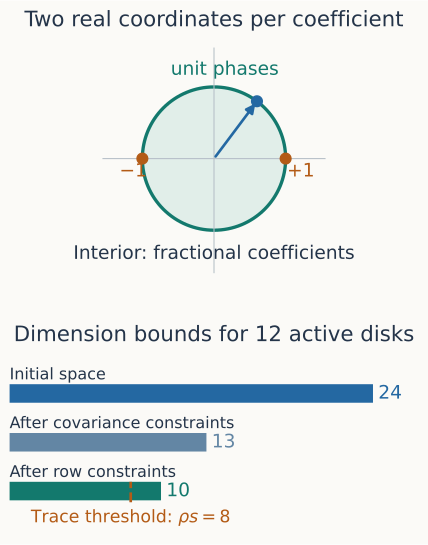
With $s=12$ active disks and the paper’s parameters, there are $24$ real coordinates. Equalizing the column derivatives costs at most $11$ dimensions, and the row-normal count costs at most $3$. At least $10$ dimensions remain, exceeding the block-trace threshold $\rho s=8$.

The block-trace lemma

Direct differentiation of ${\gamma }_I$ shows that on $Y$ the Hessian of $\mathcal{S}$ has the form $K-D$, with

$$\begin{array}{c}K⪰0,\\ D={\mathrm{diag}}_{j\in \mathcal{V}}(d_j{I}_2)⪰0,\\ \mathrm{tr}{K}_{jj}\le \rho d_j,\\ \rho =\frac{\lambda (1+2\beta {)}^2}{2\beta }.\end{array}$$

The symbols $d_j$ here are nonnegative diagonal coefficients, distinct from the row discrepancies $d_I(x)$. The estimate uses

$$\Vert \nabla z_I(x{)}_j{\Vert }_2\le |a_i(j)|(1+2\beta ),$$

which follows from $a_i(j{)}^2\le q_i$ and $\Vert x_j{\Vert }_2\le 1$.

Restricted concavity from block traces

If $K,D$ satisfy these bounds, every subspace $Y\subseteq {\mathbb{R}}^{2s}$ with $\dim Y>\rho s$ contains a nonzero $v$ such that

$$v^{T}Kv\le v^{T}Dv.$$

This is Guillen–Kobzar, Lemma 4.2. (Guillen & Kobzar, 2026)

For completeness, zero diagonal blocks of $D$ force the corresponding blocks of $K$ to vanish, by positivity and the trace bound. Thus $\ker D\subseteq \ker K$. If $Y$ meets this kernel nontrivially, use a vector in the intersection. Otherwise take a $D$-orthonormal basis of $Y$ and compare it with the positive matrix

$$B_D=D^{†/2}K{D}^{†/2},$$

where $D^{†}$ inverts positive diagonal entries and leaves zero entries zero. Its trace is

$$\begin{array}{rl}\mathrm{tr}{B}_D& =\sum _{j:d_j>0}\frac{\mathrm{tr}{K}_{jj}}{d_j}\\ & \le \rho s<\dim Y.\end{array}$$

Averaging the quadratic form over the transformed orthonormal basis gives a vector with the required inequality.

Choose parameters so that

$$\frac{4(1+\delta )}{\alpha }+\rho \le 1.$$

Then $\dim Y\ge 1+\rho s$, and the lemma supplies $v\ne 0$ with $v^T{D}^2\mathcal{S}v\le 0$. Consequently,

$$v^T{D}^2\mathcal{J}v\le -2\eta \Vert v{\Vert }_2^2<0.$$

If all active coefficients are strictly inside their disks, a short two-sided segment $x+tv$ stays feasible by the preceding constraint calculation. A twice differentiable function cannot have negative second derivative along such a segment at a local minimum. Every minimizer in the controlled potential range must therefore have an active coefficient on its boundary circle.

From the minimum principle to a complete coloring

Freezing a boundary coefficient leaves $G_i$ unchanged and reduces $q_i$. The scalar monotonicity of $z$ and $\gamma$ in $q$ preserves admissibility and does not increase $\mathcal{J}$. Transitions from a large row to an intermediate row use $d_I=0$ and $\gamma (0,G,q)<1$; rows reaching $q=0$ retain the bound $d_I\le C$.

The monotonicity follows directly from the choice of barrier. Put $\omega =\beta +2/\lambda$. Holding $d,G$ fixed with $0\le G\le q$,

$${\partial }_{q}z=\frac{\omega q-\beta G}{2q^{3/2}}\ge \frac{1}{\lambda \sqrt{q}}>0.$$

On the admissible region $z\le 0$, this gives

$$\begin{array}{rl}{\partial }_q\log \gamma & =-\frac{1}{q}+\frac{\lambda {\partial }_{q}z}{\sqrt{q}}-\frac{\lambda z}{2q^{3/2}}\\ & \ge 0.\end{array}$$

Thus reducing $q$ decreases both quantities as long as $G\le q$; compatibility ensures this even after freezing.

Minimize ${\mathcal{J}}_{\mathcal{V}}(x)$ over all admissible compatible pairs $(\mathcal{V},x)$, choosing a minimizer with the fewest active coordinates. This domain is a finite union of compact sets. It is nonempty because $(\{1,\dots ,n\},0)$ is admissible. A boundary coefficient could be frozen without increasing the objective, contradicting the choice of active set. Therefore every active coefficient of this minimizer is interior.

To put this minimizer in the potential range required above, choose

$$\tau =\frac{\delta }{2\log (en)},\eta =\frac{\delta }{2n}.$$

At $x=0$, the column normalization gives $L_j(0)\le 1$, so

$$\begin{array}{rl}{\mathcal{J}}_{[n]}(0)& ={\mathcal{S}}_{[n]}(0)\\ & \le 1+\tau \log n\le 1+\frac{\delta }{2}.\end{array}$$

Optimality and $\eta {\sum }_j\Vert x_j{\Vert }_2^2\le \delta /2$ imply ${\mathcal{S}}_{\mathcal{V}}(x)\le 1+\delta$ at the chosen minimizer. The minimum principle now contradicts any nonempty active set. Thus every coefficient has modulus one and all four directional row discrepancies are at most $C$.

The paper’s explicit parameters are

$$\begin{array}{c}\alpha =\frac{49}{4},\beta =\frac{1}{2},\lambda =\frac{1}{6},\\ C=46,\delta =\frac{1}{100},\\ \rho =\frac{2}{3},\\ \frac{4(1+\delta )}{\alpha }+\rho =\frac{3662}{3675}<1.\end{array}$$

They also satisfy $C>(2\beta +2/\lambda )\sqrt{\alpha }=45.5$, which ensures the initial barrier and contraction properties. Bounding both coordinates of each row sum by $46$ gives its Euclidean norm at most $46\sqrt{2}$.

This explains why the proof reaches phases. Replacing every disk by an interval would leave only $s$ initial dimensions; the same covariance and constraint count would no longer provide the subspace required by the block-trace lemma.

🏷️ Unitary matrices and Gaussian discrepancy

The complex viewpoint also gives a sharp special case. If $U\in {\mathbb{C}}^{n\times n}$ is unitary, every $z\in {\mathbb{T}}^n$ has

$$\Vert Uz{\Vert }_2=\Vert z{\Vert }_2=\sqrt{n},$$

so $\Vert Uz{\Vert }_{\infty }\ge 1$. Guillen–Kobzar obtain equality using the Idel–Wolf normal-form theorem: there are diagonal unitary matrices $D_1,D_2$ for which $W=D_{1}U{D}_2$ has every row and column sum equal to one. With $z=D_{2}1$,

$$Uz=D_1^{\ast }W1=D_1^{\ast }1\in {\mathbb{T}}^n.$$

Hence $\mathrm{cdisc}(U)=1$. The normal-form theorem is the external existence input; preserving Euclidean norm alone supplies only the lower bound. (Guillen & Kobzar, 2026)

For a real matrix, Gaussian discrepancy is

$$\mathrm{Gdisc}(A)=\underset{\begin{array}{c}\Sigma ⪰0\\ {\Sigma }_{jj}=1\end{array}}{\inf }{\mathbb{E}}_{G\sim N(0,\Sigma )}\Vert AG{\Vert }_{\infty }.$$

The diagonal condition requires every coordinate of $G$ to be a standard Gaussian, while allowing correlations, including singular covariance matrices. Given a planar coloring $u_j\in {\mathbb{S}}^1$, take $g\sim N(0,I_2)$ and set $G_j=⟨g,u_j⟩$. Its covariance is ${\Sigma }_{jk}=⟨u_j,u_k⟩$, and

$$\begin{array}{c}\Vert AG{\Vert }_{\infty }\le \Vert g{\Vert }_2\underset{i}{\max }{\Vert \sum _j{A}_{ij}{u}_j\Vert }_2,\\ \mathrm{Gdisc}(A)\le \sqrt{2}{\mathrm{Vdisc}}_2(A).\end{array}$$

The last step uses $\mathbb{E}\Vert g{\Vert }_2\le (\mathbb{E}\Vert g{\Vert }_2^2{)}^{1/2}=\sqrt{2}$. The phase theorem therefore gives the stated Gaussian consequence, with bound $92$ under the real column normalization.

🏷️ Consequences and the relation among the methods

For a set system $S_1,\dots ,S_d$ on $n$ elements, let $A_{ji}=1_{\{i\in S_j\}}$. If every element belongs to at most $t$ sets, each column has squared norm at most $t$. Applying the Boolean theorem to $A/\sqrt{t}$ gives, for $t\ge 1$,

$$\underset{j}{\max }\left|\sum _{i\in S_j}{\epsilon }_i\right|<3\sqrt{2\pi t}.$$

This is the square-root degree bound in the Beck–Fiala conjecture, with no restriction relating $t$ to $n$. If $t=0$, all set imbalances are zero. The elementary proof gives the same dependence with constant $36$.

The three papers provide different proof mechanisms and different permissible coefficients:

Paper	Coefficients for real inputs	Bound from its proof
Guo–Fang–Lu	Boolean signs	$<3\sqrt{2\pi }$
Karingula–Lovett	Boolean signs	$\le 36$
Guillen–Kobzar	Unit complex phases	$\le 46\sqrt{2}$

For real inputs, a Boolean signing is already a phase coloring. Consequently the first theorem also supplies the stronger numerical phase bound $3\sqrt{2\pi }$. More generally, stacking real and imaginary parts of a complex matrix and using Boolean signs gives the derived bound

$$\mathrm{cdisc}(M)<\sqrt{2}(3\sqrt{2\pi })=6\sqrt{\pi }.$$

Indeed, it simultaneously bounds the real and imaginary parts of every output coordinate by $3\sqrt{2\pi }$, and complex modulus is their Euclidean norm. Similarly, using $G=g\epsilon$ with one standard real Gaussian $g$ and a Boolean signing gives

$$\mathrm{Gdisc}(A)\le \sqrt{\frac{2}{\pi }}\mathrm{disc}(A)<6.$$

These are consequences of combining the definitions with the Boolean theorem, not the constants established by the Bellman proof. The distinctive contribution of the phase paper is its independent minimum principle and its sharp unitary example.

The overlap proofs preserve freedom through an auxiliary coordinate and then recover signs. The phase proof starts with two coordinates per coefficient and uses a dimension count to retain an admissible direction of negative curvature. In each case, the invariant must survive every operation without adding an error proportional to the number of input vectors.

Final sums, prefixes, and computational scope

The Boolean theorems control ${\sum }_{i=1}^n{\epsilon }_i{v}_i$. Controlling every fixed-order prefix with one signing asks instead for

$$\underset{1\le k\le n}{\max }{\Vert \sum _{i=1}^k{\epsilon }_i{v}_i\Vert }_{\infty }.$$

That is a stronger requirement. Karingula–Lovett’s revised introduction reports Kintali’s counterexamples with prefix discrepancy $\Omega (\sqrt{\log \log n})$, so a universal constant for all prefixes is false. Neither the extra-bit induction nor the backward geometric recovery supplies such a prefix bound. (Karingula & Lovett, 2026)

The elementary proof is a finite construction for rational input, but its growing support and extra coordinates do not establish polynomial running time. The directional-variation proof uses variationally chosen densities, and the phase proof minimizes over constrained compact sets; these are also existence arguments. A separate subsequent paper, Guo–Fang–Lu’s Vector Balancing in Polynomial Time, provides a polynomial-time constant-discrepancy signing algorithm in the unit-cost real-RAM model (Guo, Fang & Lu, 2026a). Its algorithmic result is distinct from the three proofs developed here.

See Also

Euclidean vector balancing and Steinitz orderings studies simultaneous prefixes in Euclidean norm and rearrangements of zero-sum families. The norm, permissible reordering, and prefix requirement distinguish those problems from final-sum Komlós discrepancy.

on Graham’s rearrangement conjecture develops a different exact correction mechanism: local swaps preserve one weighted sum while changing another. It provides a combinatorial counterpart to the support-preserving correction of a mean used here.

🐻  Guillen, N. & Kobzar, V.A. 2026. The Komlós conjecture for complex discrepancy.

🐻  Guo, S., Fang, E.X. & Lu, J. 2026a. Vector Balancing in Polynomial Time.

🐻  Guo, S., Fang, E.X. & Lu, J. 2026b. Vector Balancing via Directional Total Variation.

🐻  Karingula, S.R. & Lovett, S. 2026. An elementary proof of the Komlós conjecture.