on diffusion models

Overview

This post serves as a study note for diffusion-based generative models. It explores the transition from the ill-posed inverse heat equation to the stable reverse-time SDE framework and the mechanism of denoising score matching.

🏷️ Introduction

The diffusion model implements an encode/decode process through the gradual addition and removal of Gaussian noise. Mathematically, this is framed as a transition from a complex data distribution $p_0(x)$ to a simple prior (usually standard Gaussian) $p_T(x)$, and then learning the reverse trajectory.

🏷️ The Forward Process: Diffusion and Entropy

The process of adding noise can be modeled by a Forward Stochastic Differential Equation (SDE):

$$d{X}_t=f(x,t)dt+g(t)d{W}_t$$

where $f(x,t)$ is the drift coefficient and $g(t)$ is the diffusion coefficient. The evolution of the probability density $p_t(x)$ is governed by the Fokker-Planck Equation:

$$\frac{\partial p_t(x)}{\partial t}=-\nabla \cdot [f(x,t)p_t(x)]+\frac{1}{2}g(t{)}^2\Delta p_t(x)$$

As $t\to T$, the initial data distribution “diffuses” and converges to a stationary Gaussian distribution.

🏷️ The Challenge: The Ill-Posed Inverse Problem

Intuitively, “denoising” sounds like solving the Inverse Heat Equation. In its simplest form ($f=0,g=1$), reversing time $\tau =T-t$ leads to:

$$\frac{\partial p}{\partial \tau }=-\frac{1}{2}\Delta p$$

This is a classic ill-posed problem in numerical analysis. The inverse heat operator is unbounded, meaning that high-frequency components (noise) are amplified exponentially.

In a diffusion model, this instability doesn’t disappear; it is “packed” into the Score Term. If we were to attempt the reverse process without a precise guide, any small error in the trajectory would explode. The ill-posedness of the inverse PDE is the reason why naive “un-mixing” or “de-blurring” fails.

🏷️ The Solution: Score-Based Reverse SDE

The breakthrough (Anderson, 1982) is that the time-reversal of a diffusion process is itself a diffusion process, provided we have access to the Score Function $\nabla \log p_t(x)$.

The Reverse-Time SDE is given by:

$$d{X}_t=[f(x,t)-g(t{)}^2\nabla \log p_t(x)]dt+g(t)d{\bar{W}}_t$$

Stability via Guidance

The term $-g(t{)}^2\nabla \log p_t(x)$ acts as a vector field that points toward regions of higher data density.

1. Regularization: The score term explicitly provides the information “lost” to entropy during the forward process. It effectively transforms the ill-posed PDE inversion into a stable, guided stochastic process.
2. Noise as a Prior: By adding noise during the forward process, we ensure $p_t$ has full support (is non-zero everywhere). This “smears” the data manifold, making the score function a smooth, learnable vector field instead of a singular one.

🏷️ The Neural “Trick”: Denoising Score Matching

The primary difficulty is that $p_t(x)$ is unknown. However, we can bypass this using Denoising Score Matching (DSM). The core idea is that while we don’t know the global score $\nabla \log p_t(x_t)$, we know the conditional score $\nabla \log p(x_t|x_0)$ because we know the noise we added.

A fundamental identity shows that the gradients of these two objectives are the same:

$${\mathbb{E}}_{x_t\sim p_t}[\Vert s_{\theta }(x_t,t)-\nabla \log p_t(x_t){\Vert }^2]={\mathbb{E}}_{x_0,x_t}[\Vert s_{\theta }(x_t,t)-\nabla \log p(x_t|x_0){\Vert }^2]$$

Since $p(x_t|x_0)$ is a Gaussian transition (e.g., $x_t=\sqrt{{\alpha }_t}{x}_0+\sqrt{1-{\alpha }_t}ϵ$), its score is simply:

$${\nabla }_{x_t}\log p(x_t|x_0)=-\frac{x_t-\sqrt{{\alpha }_t}{x}_0}{1-{\alpha }_t}$$

Insight: We trade a hard numerical integration problem (Inverse Heat Eq) for a high-dimensional interpolation problem (Neural Score Estimation). The network doesn’t “invert the PDE”; it learns a prior from millions of forward paths, allowing it to “hallucinate” the most likely denoised state.

📊 Numerical Verification

To illustrate these concepts, consider a 2D point cloud generated from a “Swiss Roll” distribution. We implemented a simple diffusion model using PyTorch (see content/codes/2025 Summer/diffusion_swissroll.py).

1. Forward Process: Gradually corrupt the 2D Swiss roll with Gaussian noise according to a linear variance schedule ${\beta }_t$.
2. Score Estimation: Train a multi-layer perceptron (MLP) to predict the noise $ϵ$ added at each step $t$. This is equivalent to estimating the score function $\nabla \log p_t(x_t)$.
3. Reverse Sampling: Starting from pure Gaussian noise, iteratively subtract the estimated noise to recover the original distribution.

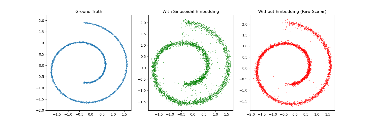
(Above: A comparison between ground truth, samples generated with sinusoidal embeddings, and samples generated with raw scalar time input. In many 2D cases, the simpler scalar input yields a smoother, more stable result.)

🏷️ Notes

• The stability of the reverse SDE depends heavily on the accuracy of the score estimation, especially in low-density regions.
• Stochastic vs Deterministic: One can also define a Probability Flow ODE that shares the same marginal densities as the SDE but is deterministic: $dx=[f-\frac{1}{2}{g}^2\nabla \log p_t]dt$.

🔗 See Also

• on Ising models
• on improved Nyström bounds

📚 References