on convergence of graph Laplacian to manifold's Laplacian

Info

This post is more like an exercise for personal interest. It does not necessarily contain anything new.

🏷️Introduction

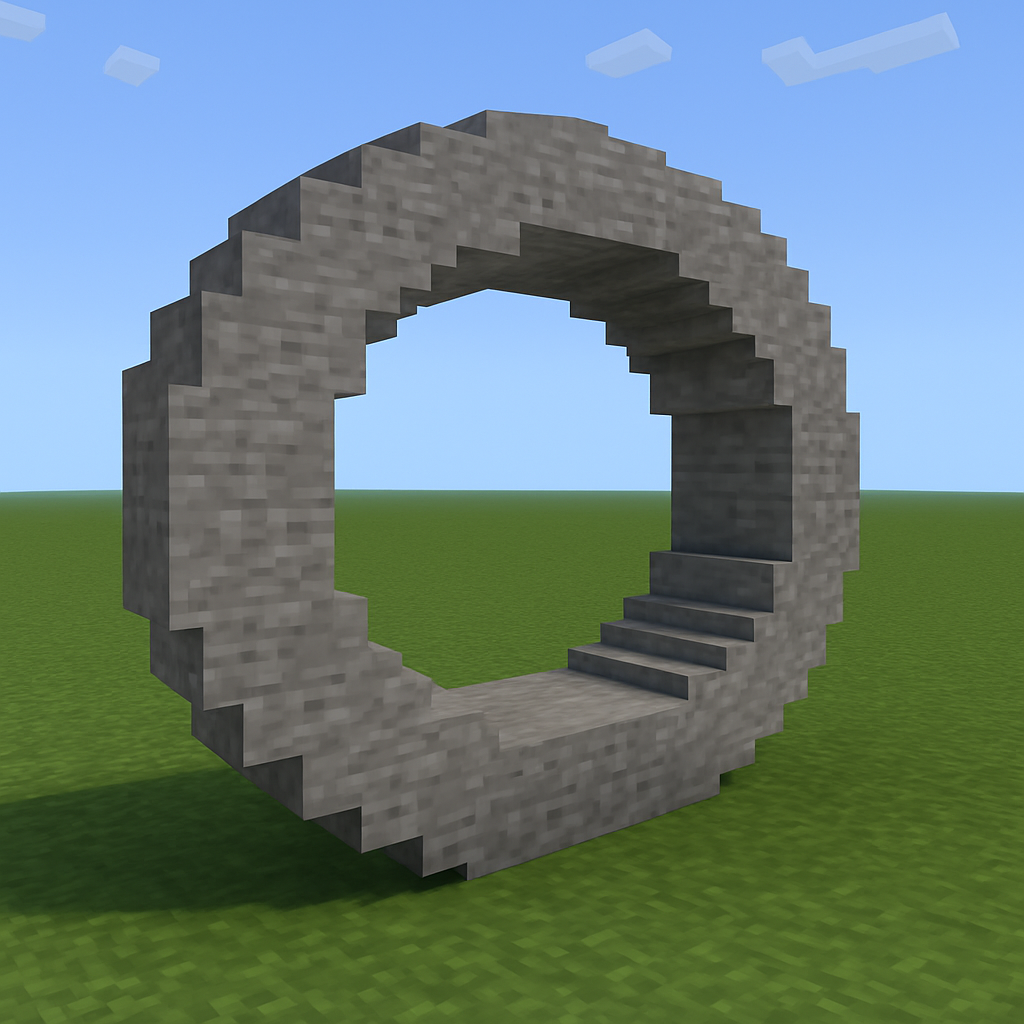
Let us imagine that a closed smooth manifold is constructed in Minecraft😅, we can expect some detailed information is likely to lose.

Image source: ChatGPT

So, it is natural to ask:

How much geometric information is still kept?

Intuitively, we may find the smooth part is still recognizable while the details will be gone. In the following, we try to make this rigorous. The whole idea is to show the spectrum of the graph Laplacian derived from the lattice converges to the spectrum of the smooth manifold’s Laplacian, to certain extent.

❕Story time!

Let $\Gamma \subset {\mathbb{R}}^3$ be a smooth, closed, oriented surface. Denote ${\Delta }_{\Gamma }$ the Laplace-Beltrami operator on $\Gamma$ and ${\nabla }_{\Gamma }$ be the gradient operator. We also denote $\{{\varphi }_k{\}}_{k\ge 0}$ as the eigenfunctions of $-{\Delta }_{\Gamma }$ with corresponding eigenvalues $\{{\lambda }_k{\}}_{k\ge 0}$. The first trivial eigenvalue ${\lambda }_0=0$.

Our story starts with something between the Minecraft (lattice graph) and the manifold.

🌵Eigenvalue estimates in tube

Let $d_{\Gamma }$ denote the signed distance function to $\Gamma$ that takes the negative sign for points inside the region enclosed by $\Gamma$. With the distance function to $\Gamma$, the projection operator can be evaluated by

$$P_{\Gamma }(x):=x-d_{\Gamma }(x)\nabla d_{\Gamma }(x).$$

The projection operator is well-defined when the $|d_{\Gamma }(x){|}^{-1}$ is larger than the maximum principal curvature of $\Gamma$.

Definition

Let ${\Gamma }_t$ be the level set

$${\Gamma }_t:=\{x\in {\mathbb{R}}^3\mid d_{\Gamma }x=t\}$$

and the tube $D_t:=\{x\in {\mathbb{R}}^3\mid |d_{\Gamma }x|<t\}$

Then we prove the following lemma, which shows the eigenvalues of the Laplacian on $D_r$ can approximate the eigenvalues of ${\Delta }_{\Gamma }$ as the tube width $r\ll 1$.

Lemma

Let $r>0$ be a small parameter. Assume that ${\psi }_0,{\psi }_1,\cdots$ are the eigenfunctions of the following eigenvalue problem with Neumann boundary condition

$$\begin{array}{rlrl}-\Delta {\psi }_k& ={\mu }_k{\psi }_k& \text{ in }& D_r\\ \frac{\partial {\psi }_k}{\partial n}& =0& \text{ on }& \partial D_r.\end{array}$$

Then there exists a constant $C>0$ independent of $r$ that $|{\lambda }_k-{\mu }_k|\le Cr{\lambda }_k$.

Proof of lower bound

The main tool is the min-max principle,

$${\mu }_k=\underset{\dim U=k+1}{\min }\underset{f\in U-\{0\}}{\max }\frac{{\int }_{D_r}|\nabla f(x){|}^{2}dx}{{\int }_{D_r}|f(x){|}^{2}dx}.$$

We first provide a lower bound for ${\mu }_k$. Our estimate consists of three steps.

Step 1: Explicit construction of the subspace $U$. We define the functions $\{h_m{\}}_{m=0}^k$ by

$$h_m(x)={\varphi }_m(P_{\Gamma }x).$$

and denote $U=\mathrm{span}(h_0,\cdots ,h_k)$.

Step 2: Estimate of norms. Let $f\in U$, and we apply the co-area formula

$$\begin{array}{rl}{\int }_{D_r}|f(x){|}^{2}dx& ={\int }_{-r}^r{\int }_{d_{\Gamma }(x)=t}|f(x){|}^{2}dSdt\\ & ={\int }_{-r}^r{\int }_{d_{\Gamma }(x)=t}|f(P_{\Gamma }x){|}^{2}dSdt\end{array}$$

Let $J(x)$ be the Jacobian between the surfaces $\{d_{\Gamma }=t\}$ and $\Gamma$, then

$${\int }_{d_{\Gamma }(x)=t}|f(P_{\Gamma }x){|}^{2}J(x)dS={\int }_{\Gamma }|f(x){|}^{2}dS$$

where $J(x)=1-d_{\Gamma }(x)\Delta d_{\Gamma }(x)+|d_{\Gamma }(x){|}^2⟨\nabla d_{\Gamma },{\nabla }^2{d}_{\Gamma }\nabla d_{\Gamma }⟩$.

Therefore, $J(x)=1+O(r)$, we have the following estimate

$${\int }_{D_r}|f(x){|}^{2}dx=2r\left(1+O(r)\right){\int }_{\Gamma }|f(x){|}^{2}dS.$$

We then estimate

$$\begin{array}{rl}{\int }_{D_r}|\nabla f{|}^{2}dx& ={\int }_{-r}^r{\int }_{d_{\Gamma }(x)=t}|\nabla f(x){|}^{2}dSdt\\ & ={\int }_{-r}^r{\int }_{d_{\Gamma }(x)=t}|\nabla f(P_{\Gamma }x){|}^{2}dSdt=2r(1+O(r)){\int }_{\Gamma }|\nabla f(x){|}^{2}dS\\ & =2r(1+O(r)){\int }_{\Gamma }|{\nabla }_{\Gamma }f(x){|}^{2}dS.\end{array}$$

Step 3: Apply the min-max principle.

$$\begin{array}{rl}{\mu }_k& \le (1+O(r))\underset{f\in U-\{0\}}{\max }\frac{{\int }_{\Gamma }|{\nabla }_{\Gamma }f(x){|}^{2}dS}{{\int }_{\Gamma }|f(x){|}^{2}dS}\\ & =(1+O(r)){\lambda }_k.\end{array}$$

Proof of upper bound

Next, we provide an upper bound estimate using the max-min counterpart.

$${\mu }_k=\underset{\dim U=k}{\max }\underset{f\in U^{\perp }-\{0\}}{\min }\frac{{\int }_{D_r}|\nabla f(x){|}^{2}dx}{{\int }_{D_r}|f(x){|}^{2}dx}.$$

Step 4: Explicit construction of $U$. We define the functions $\{w_m{\}}_{m=0}^{k-1}$ by

$$w_m(x)=\sqrt{\mathcal{J}(x)}{\varphi }_m(P_{\Gamma }x),\mathcal{J}(x):=\frac{J(x)+J(2P_{\Gamma }x-x)}{2}.$$

where $2P_{\Gamma }x-x$ is the mirror point of $x$ across $\Gamma$. Then for $\forall i\ne j$, using the symmetry of the domain along normal direction,

$$\begin{array}{rl}{\int }_{D_r}{w}_i(x)w_j(x)dx& ={\int }_{-r}^r{\int }_{d_{\Gamma }(x)=t}{w}_i(x)w_j(x)dSdt\\ & ={\int }_{-r}^r{\int }_{d_{\Gamma }(x)=t}{\varphi }_i(P_{\Gamma }x){\varphi }_j(P_{\Gamma }x)\mathcal{J}(x)dSdt\\ & ={\int }_{-r}^r{\int }_{d_{\Gamma }(x)=t}{\varphi }_i(P_{\Gamma }x){\varphi }_j(P_{\Gamma }x)J(x)dSdt\\ & =2r{\int }_{\Gamma }{\varphi }_i(P_{\Gamma }x){\varphi }_j(P_{\Gamma }x)dS=0.\end{array}$$

which implies $\{w_m{\}}_{m=0}^{k-1}$ forms an orthogonal set and let $U=\text{span}(w_0,\cdots ,w_{k-1})$.

Step 5: Norm estimates are similar to the previous case. For $f\in U$, we can write $f(x)=\sqrt{\mathcal{J}(x)}\tilde{f}(x)$ that $\tilde{f}\in \text{span}(h_0,\cdots ,h_m)$ and

$${\int }_{d_{\Gamma }(x)=t}|f(x){|}^{2}dS={\int }_{\Gamma }|\tilde{f}(x){|}^{2}dS.$$

which implies

$${\int }_{D_r}|f(x){|}^{2}dx=2r{\int }_{\Gamma }|\tilde{f}(x){|}^{2}dS.$$

In a similar spirit, we have

$$\begin{array}{rl}{\int }_{D_r}|\nabla f{|}^{2}dx& ={\int }_{-r}^r{\int }_{d_{\Gamma }(x)=t}|\nabla f(x){|}^{2}dSdt\\ & ={\int }_{-r}^r{\int }_{d_{\Gamma }(x)=t}{\left|\sqrt{\mathcal{J}(x)}\nabla \tilde{f}(P_{\Gamma }x)+\tilde{f}(x)\nabla \sqrt{\mathcal{J}(x)}\right|}^{2}dSdt.\end{array}$$

By cancellation, $\mathcal{J}(x)=1+O(r^2)$, which implies that $\sqrt{\mathcal{J}(x)}=1+O(r^2)$ and $|\nabla \sqrt{\mathcal{J}(x)}|=O(r)$ as well. Therefore,

$${\int }_{D_r}|\nabla f{|}^{2}dx=2r\left((1+O(r)){\int }_{\Gamma }|{\nabla }_{\Gamma }f{|}^{2}dS+O(r){\int }_{\Gamma }|f{|}^{2}dS\right).$$

Step 6: We will now use the max-min principle

$$\begin{array}{rl}{\mu }_k& \ge \underset{f\in U^{\perp }-\{0\}}{\min }\frac{(1+O(r)){\int }_{\Gamma }|{\nabla }_{\Gamma }f(x){|}^{2}dS+O(r){\int }_{\Gamma }|f(x){|}^{2}dS}{{\int }_{\Gamma }|f(x){|}^{2}dS}\end{array}$$

For $k\ge 1$, since ${\varphi }_0$ is a constant function, we have ${\int }_{\Gamma }f(x)dS=0$, then by the Poincaré inequality, there exists a constant $C^{\prime }>0$ that

$${\int }_{\Gamma }|{\nabla }_{\Gamma }f{|}^{2}dS\ge C^{\prime }{\int }_{\Gamma }|f{|}^{2}dS.$$

Thus we have

$$\begin{array}{rl}{\mu }_k& \ge \underset{f\in U^{\perp }-\{0\}}{\min }\frac{(1+O(r)){\int }_{\Gamma }|{\nabla }_{\Gamma }f(x){|}^{2}dS+O(r){\int }_{\Gamma }|{\nabla }_{\Gamma }f{|}^{2}dS}{{\int }_{\Gamma }|f(x){|}^{2}dS}\\ & =(1+O(r)){\lambda }_k.\end{array}$$

Notes

Links